10.4 A Concluding Application
Let us return again to our analysis on the median starting salaries of graduating law classes by adding a dummy variable that replaces our original measure of school quality.
\[SALARY_i = \beta_0 + \beta_1 \; LSAT_i + \beta_2 \; TOP25_i + \varepsilon_i\]
where…
\(TOP25_i = 1\) if school i is ranked in the top 25
\(TOP25_i = 0\) if school i is ranked 26 or higher
The model above replaced the rank of each school with an indicator variable breaking the schools into two categories: the top 25 best schools and all the rest. This switch makes the assumption that there is a more broad impact of school quality. In other words, there is no difference between the top school and any other school in the top 25, but there is a difference between this top 25 and the rest.
##
## Call:
## lm(formula = SALARY ~ LSAT + TOP25, data = LAW)
##
## Residuals:
##    Min     1Q Median     3Q    Max
## -11002  -3888   -293   3075  21187
##
## Coefficients:
##              Estimate Std. Error t value Pr(>|t|)
## (Intercept) -107398.9    20260.4  -5.301 4.42e-07 ***
## LSAT            903.1      129.1   6.998 1.01e-10 ***
## TOP25         20188.5     1590.9  12.690  < 2e-16 ***
## ---
## Signif. codes:  0 '***' 0.001 '**' 0.01 '*' 0.05 '.' 0.1 ' ' 1
##
## Residual standard error: 5601 on 139 degrees of freedom
## Multiple R-squared:  0.7939, Adjusted R-squared:  0.7909
## F-statistic: 267.6 on 2 and 139 DF,  p-value: < 2.2e-16
Interpretations are as follows:
\[\hat{\beta}_1 = \frac{\Delta \widehat{SALARY}}{\Delta LSAT} = 903.14\]
Holding \(TOP25\) constant, one additional LSAT point will result in a $903.14 increase in median starting salary on average. Note that holding TOP25 constant implies that we are making no distinction between graduates inside and outside of the top 25. This coefficient is isolating the impact of LSAT score.
\[\hat{\beta}_2 = \frac{\Delta \widehat{SALARY}}{\Delta TOP25} = 20188.51\]
Holding \(LSAT\) constant, graduating from a top 25 school will result in a $20188.51 increase in median starting salary (than graduating from a non-top 25 school) on average. Note that this coefficient is isolating the impact of moving from outside the top 25 (i.e., the zero category) to inside the top 25 (i.e., the one category).
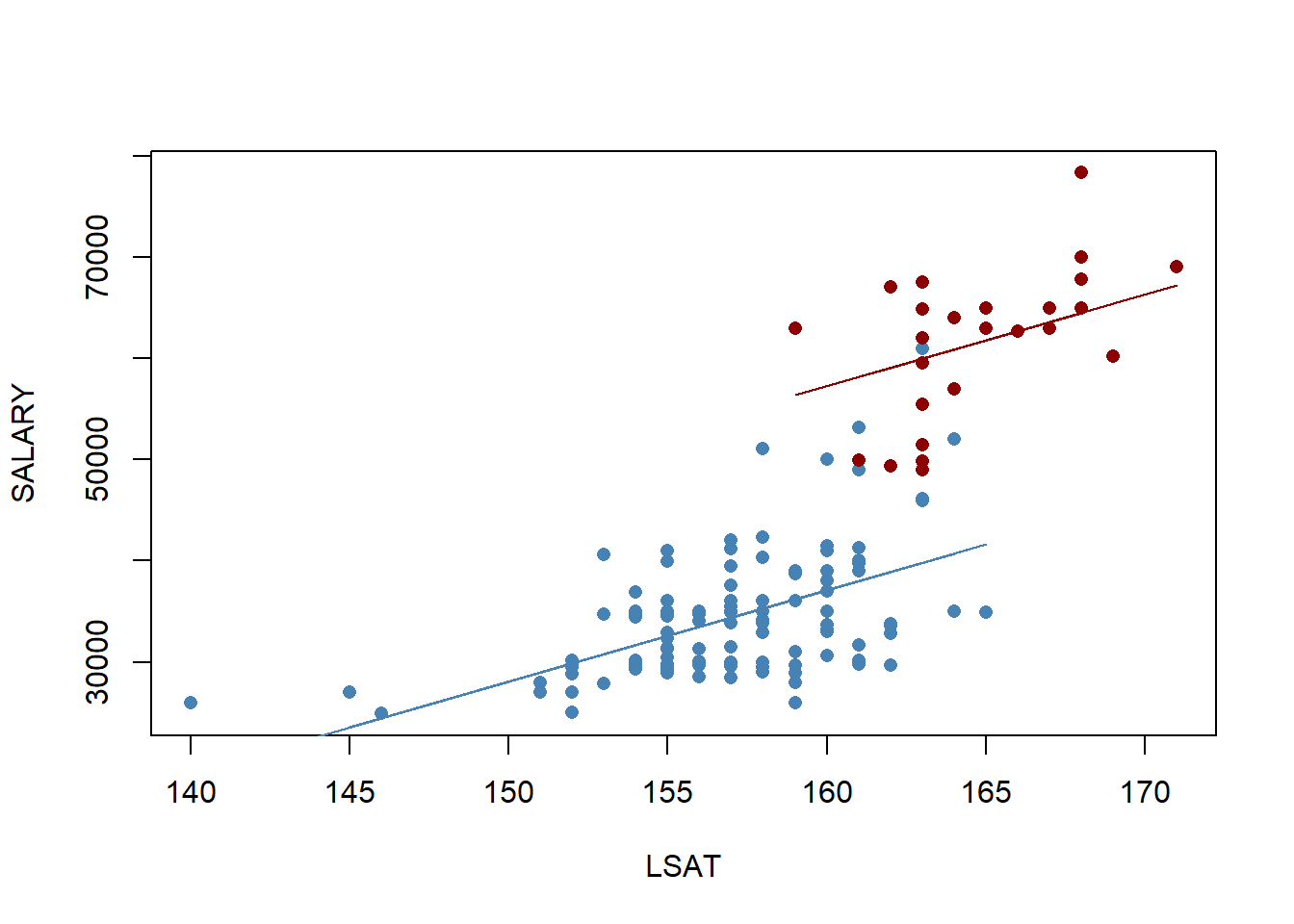
The figure below illustrates why this type of dummy variable is called an intercept dummy. The figure shows the relationship in the data between the median starting salary and the average LSAT score, only the red dots indicate data observations from within the top 25 law schools while the blue dots indicate data observations outside of the top 25. The regression line for the top 25 schools is parallel to the regression line for the rest of the schools (by design), but is simply elevated by the value of the coefficient in front of the dummy variable. This means that the dummy variable increased the intercept of the regression line by 20188.51.
We can extend this analysis to test the assumption implicitly made by our model: does an extra LSAT point impact starting salary differently if a student is in the top 25?
\[SALARY_i = \beta_0 + \beta_1 \; LSAT_i + \beta_2 \; TOP25_i + \beta_3 \; (LSAT_i \times TOP25_i) + \varepsilon_i\]
Our slope dummy is a specific example of an interaction term (which is simply a new independent variable being the product of two existing independent variables). An interaction term allows the two slopes to impact each other in a very straightforward way.
##
## Call:
## lm(formula = SALARY ~ LSAT + TOP25 + I(LSAT * TOP25), data = LAW)
##
## Residuals:
##      Min       1Q   Median       3Q      Max
## -10128.4  -3790.5   -595.8   2922.8  21550.2
##
## Coefficients:
##                 Estimate Std. Error t value Pr(>|t|)
## (Intercept)     -97981.4    21358.6  -4.587 9.97e-06 ***
## LSAT               843.1      136.1   6.197 6.23e-09 ***
## TOP25           -72884.6    68616.5  -1.062    0.290
## I(LSAT * TOP25)    567.9      418.5   1.357    0.177
## ---
## Signif. codes:  0 '***' 0.001 '**' 0.01 '*' 0.05 '.' 0.1 ' ' 1
##
## Residual standard error: 5584 on 138 degrees of freedom
## Multiple R-squared:  0.7966, Adjusted R-squared:  0.7921
## F-statistic: 180.1 on 3 and 138 DF,  p-value: < 2.2e-16
To see if an additional LSAT point has a different impact inside or outside of the top 25, we examine the coefficient infront of the LSAT variable as well as the partial derivative of the interaction term.
\[\frac{\Delta \widehat{SALARY}}{\Delta LSAT} = \hat{\beta}_1 + \hat{\beta}_3 \; TOP25\]
Recall that \(TOP25\) takes on a value of 1 if the school is in the top 25 schools (0 otherwise).
If \(TOP25 = 0\):
\[\frac{\Delta \widehat{SALARY}}{\Delta LSAT} = \hat{\beta}_1 + \hat{\beta}_3 \times 0 = 843.14\]
If \(TOP25 = 1\):
\[\frac{\Delta \widehat{SALARY}}{\Delta LSAT} = \hat{\beta}_1 + \hat{\beta}_3 \times 1 = 843.14 + 567.87\]
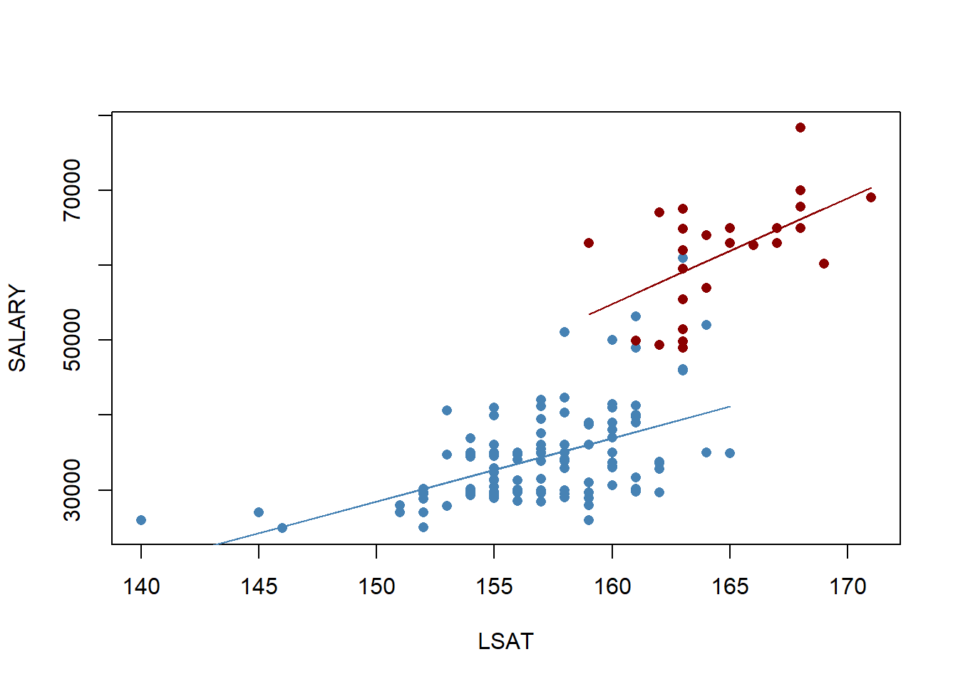
According to our estimates, an additional LSAT point has a larger impact of about $568 if the law student was in the top 25 schools. This means that the slope with respect to LSAT is 568 higher, as the figure below illustrates.
\[H_0: \beta_3 = 0 \quad vs \quad H_1: \beta_3 \neq 0\]
Of course, while our sample suggests that students from the top 25 benefit more from an additional LSAT point, the main concern is what we think is happening in the population. The p-value for our slope dummy variable is 0.177, indicating that we cannot reject the null hypothesis stating that \(\beta_3\) is not significantly different from zero (at 90% confidence or better). This ultimately suggests that our first model that assumed there was no interaction between LSAT and TOP25 is actually the more appropriate model. What we gained by extending the model and showing that the extension wasn’t necessary is that we have more confidence that our intercept dummy variable model is closer to true model.