12.4 A Concluding Application
Let us turn one final time to our analysis of the starting salaries of law students. In our chapter on dummy variables, we made the coarse distinction between school ranks inside and outside of the top 25 schools only. Suppose we make this distinction a bit finer.
\[SALARY_i = \beta_0 + \beta_1 \; LSAT_i + \beta_2 \; TOP10_i + \beta_3 \; R11\_25_i + \varepsilon_i\]
where…
\(TOP10_i = 1\) if school i is ranked in the top ten (0 otherwise)
\(R11\_25_i = 1\) if school i is ranked 11 to 25 (0 otherwise)
benchmark… all schools ranked 26 or higher!
Note that this application is actually one where we have three qualitative categories (top 10, top 11-15, and all the rest). These three categories can be captured by two dummy variables, with schools not ranked in the top 25 serving as the benchmark category.
| Estimate | Std. Error | t value | Pr(>|t|) | |
|---|---|---|---|---|
| (Intercept) | -95057 | 20594 | -4.616 | 8.865e-06 |
| LSAT | 824.5 | 131.2 | 6.285 | 4.015e-09 |
| TOP10 | 24117 | 2275 | 10.6 | 1.432e-19 |
| R11_25 | 18589 | 1703 | 10.91 | 2.229e-20 |
| Observations | Residual Std. Error | \(R^2\) | Adjusted \(R^2\) |
|---|---|---|---|
| 142 | 5510 | 0.802 | 0.7977 |
Estimating our regression allows us to quantify the impact of graduating from a top 10 school (relative to a 26+ school) and differentiating it from the impact of graduating from a 11-25 school (relative to a 26+ school). Formal interpretations are as follows.
\[\frac{\Delta \widehat{SALARY}}{\Delta TOP10} = 24116.51\]
Holding LSAT constant, graduating from a top 10 school (relative to a school ranked 26 or lower) will result in $24116.51 in additional median starting salary, on average.
\[\frac{\Delta \widehat{SALARY}}{\Delta R11\_25} = 18589.5\]
Holding LSAT constant, graduating from a school ranked between 11-25 (relative to a school ranked 26 or lower) will result in $18589.5 in additional median starting salary, on average.
The big difference between this regression model and the one we estimated in our dummy variable chapter is that the previous model implicitly assumed that the impact of graduating from a top 10 or top 11-25 school was the same (because we only considered top 25). This model relaxed that assumption and considered two potentially different impacts. The question remains: is this refinement necessary? In other words, is there a significant difference between top 10 and top 11-25 in the population?
We can test this by way of a joint hypothesis test:
\[H_0: \beta_2 = \beta_3 \quad vs \quad H_1: \beta_2 \neq \beta_3\]
The null hypothesis states that the two slope coefficients are the same, while the alternative states that they are different. Remember this boils down to simply saying that there is no difference between top 10 and top 11-25 (under the null).
Step 1: Estimate the unrestricted model.
This is the model where the coefficients can be whatever R says they should be. We actually already did this above, so we just need to collect the unrestricted \(R^2\).
## [1] 0.8019693Step 2: Estimate the restricted model.
This is the step where we need to construct and estimate the model with the null hypothesis imposed. Since the restriction under the null is \(\beta_2 = \beta_3\), we simply set \(\beta_2\) to be the same as \(\beta_3\) and combine terms.
\[SALARY_i = \beta_0 + \beta_1 \; LSAT_i + \beta_2 \; TOP10_i + \beta_3 \; R11\_25_i + \varepsilon_i\]
\[SALARY_i = \beta_0 + \beta_1 \; LSAT_i + \beta_3 \; TOP10_i + \beta_3 \; R11\_25_i + \varepsilon_i\]
\[SALARY_i = \beta_0 + \beta_1 \; LSAT_i + \beta_3 (TOP10_i + R11\_25_i) + \varepsilon_i\]
Once we determine what the restricted model looks like on paper, we simply estimate it and collect the restricted \(R^2\).47
## [1] 0.7938553Step 3: Calculate an F-Statistic under the null
\[F_{stat} = \frac{(R^2_u - R^2_r)/m}{(1-R^2_u)/(n-k-1)}\]
Our one restriction results in \(m=1\), while \(n-k-1\) from the unrestricted model is easy to determine. These two degrees of freedom combined with our restricted and unrestricted \(R^2s\) is all we need to calculate our F statistic under the null.
## [1] 5.654371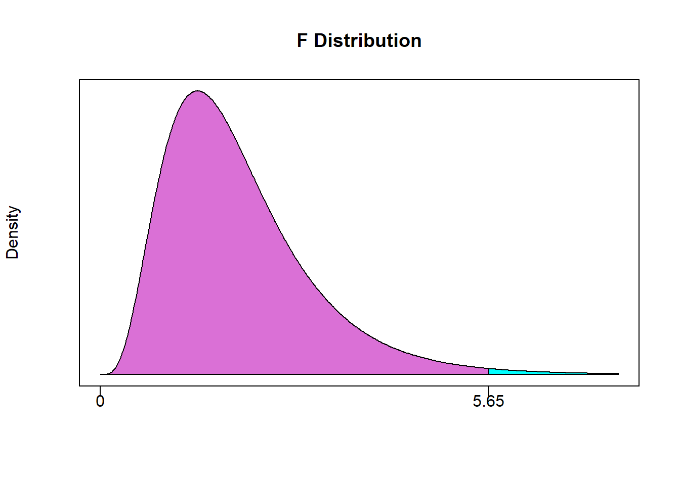
Step 4: Calculate a p-value and conclude
## [1] 0.01878279## [1] 98.12172Our p-value states that we can reject the null with 98.12 percent confidence.
This tells us that we can reject the hypothesis that graduation from the top 10 schools is the same as graduating from the top 25 (with over 98% confidence).
Think about the following. TOP10 is a column that has a 1 if the school is in the top 10 (zero otherwise), while R11_25 is a column that has a 1 if the school is ranked 11 through 25 (zero otherwise). This directly implies that the sum of these two columns now delivers a column that has a 1 if the school is ranked 1 through 25 (zero otherwise), which is identical to the top 25 variable we considered earlier.↩︎