10.1 Intercept dummy variable
An intercept dummy variable is a qualitative variable that stands alone in a regression just like other quantitative variables we have encountered. Let us illustrate this by adding an intercept dummy variable to a wage analysis.
Suppose you are a consultant hired by a firm to help determine the underlying features of the current wage structure for their employees. You want to understand why some individuals have wage rates that are different from others. Let our dependent variable be wage (the hourly wage of an individual employee) and the independent variables be given by…
educ is the total years of education of an individual employee
exper is the total years of experience an individual employee had prior to starting with the company
tenure is the number of years an employee has been working with the firm.
These independent variables are all quantitative because they directly translate to numbers. We can also add a qualitative variable to this list of independent variables to see if gender can help explain why some people earn a higher wage than others. In particular, consider the qualitative variable female which equals 1 if the individual is female and 0 if the individual is not (i.e., male).
The specified model (the PRF) now becomes
\[wage_i=\beta_0+\beta_1educ_i+\beta_2exper_i+\beta_3tenure_i+\beta_4female_i+\varepsilon_i\]
Note that the slope of the three quantitative variables are completely standard. The slope with respect to the dummy variable is similar, but needs to be interpreted in a specific manner. In particular, since we normally interpret slopes with respect to a unit increase in the independent variable, and the fact that a dummy variable can only go up one unit (i.e., from 0 to 1), we therefore interpret a dummy variable accordingly.
\[\beta_4 = \frac{\Delta wage}{\Delta female}\]
Holding education, tenure, and experience constant, a female earns a \(\beta_4\) difference in wage relative to a male, on average
Note that the dummy variable is constructed such that males receive a 0 while females receive a 1. This implies that \(\beta_4\) will denote the average change in a female’s wage relative to a male’s wage. If \(\beta_4 < 0\), then this would imply that a female’s average wage is less than a male’s.
After loading the wage1 data directly from the wooldridge package (see code below), the four independent variables are illustrated in the scatter plots below. Notice that even though the dummy variable takes on only two numbers by design, we can still see how it effectively splits the observations into the two groups.
data(wage1, package = "wooldridge")

par(mfrow = c(4,1))
plot(wage1$educ,wage1$wage,
          col = "blue", pch = 19, cex = 1,
          xlab = "Education", ylab = "Wage")
plot(wage1$exper,wage1$wage,
          col = "red", pch = 19, cex = 1,
          xlab = "Experience", ylab = "Wage")
plot(wage1$tenure,wage1$wage,
          col = "green", pch = 19, cex = 1,
          xlab = "Tenure", ylab = "Wage")
plot(wage1$female,wage1$wage,
          col = "orange", pch = 19, cex = 1,
          xlab = "Female (1 if yes)", ylab = "Wage")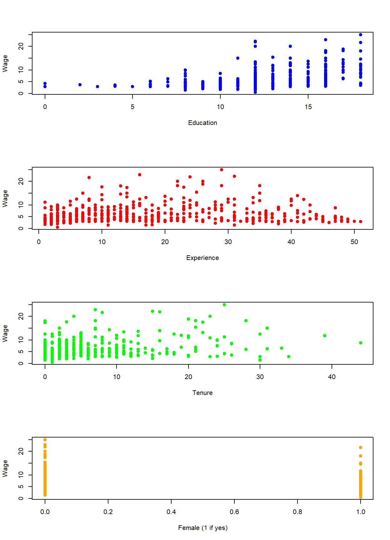
There is no difference between estimating quantitative and qualitative variables as far as R in concerned.
## (Intercept)        educ       exper      tenure
## -2.87273482 0.59896507 0.02233952 0.16926865## (Intercept) educ exper tenure female
## -1.56793870 0.57150477 0.02539587 0.14100506 -1.81085218Interpretations of the other independent variables are unchanged. However, \(\hat{\beta}_4 = -1.81\) suggests the following:
Holding education, tenure, and experience constant, a female earns $1.81 less in wages relative to a male, on average
This states that we can compare two individuals with the same education, experience, and tenure levels, but differ in gender and conclude that the male earns more.
Let us examine this further to show exactly why this type of qualitative variable is called an intercept dummy variable. Since the dummy variable can only take on the values 1 or 0, we can write down the PRF for both cases. In particular, the PRF for a male has \(female_i = 0\) while the PRF for a female has \(female_i = 1\).
\[PRF: wage_i=\beta_0+\beta_1educ_i+\beta_2exper_i+\beta_3tenure_i+\beta_4female_i+\varepsilon_i\]
\[Male: wage_i=\beta_0+\beta_1educ_i+\beta_2exper_i+\beta_3tenure_i+\varepsilon_i\] \[Female: wage_i=(\beta_0+\beta_4)+\beta_1educ_i+\beta_2exper_i+\beta_3tenure_i+\varepsilon_i\]
Notice that \(\beta_4\) does not appear in the PRF for males because the female variable equals 0, while it appears alone in the PRF for females because the female variable equals 1. After rearranging a bit, you can see that the intercept term of the PRF for males is \(\beta_0\) while the intercept term of the PRF for females is \((\beta_0+\beta_4)\). This illustrates that if you hold the other three independent variables constant, the difference between the wage rates of a male and female is \(\beta_4\) on average. In other words, if you plug in the same numbers for education, experience, and tenure in the two PRFs above, then the difference in wages between men and women who share these traits will be \(\beta_4\).