11.6 Conclusion
This section introduced you to three different ways of adding potential non-linear relationships into our model while still preserving linearity in the coefficients. This allows us to retain our OLS estimation procedure, and only requires some calculus steps after estimation to get at our answers.
One take away is that one can easily map out a functional form in theory, but it might not be entirely captured by the data sample. In other words, while we can always tell a story that a relationship might become non-linear eventually, if that extreme range is not in the data then a non-linear relationship isn’t necessary.
On the other hand, if there is a non-linear relationship in the data, then it might be the case that more than one functional form might fit. While it is true that the three transformations handle different right-side behaviors, notice that the left-side of the relationships look quite similar.
Take the figure below for example. We do not have enough data to see if the relationship stays increasing (requiring a log transformation), changes direction (requiring a quadratic transformation), or dies out (requiring a reciprocal transformation). If this is the case then trial and error combined with a lot of care is required.
Which model has the highest \(R^2\)? (Provided that the dependent variable is not transformed.)
Which model makes the most sense theoretically?
What is the differences in the out-of-sample forecasts between models? What is the cost of being wrong?
X <- seq(0,45,1)
Y <- 100 * X - X^2

plot(X,Y,
     main = "Which Relationship is This?",
     xlab = "X",
     ylab = "Y")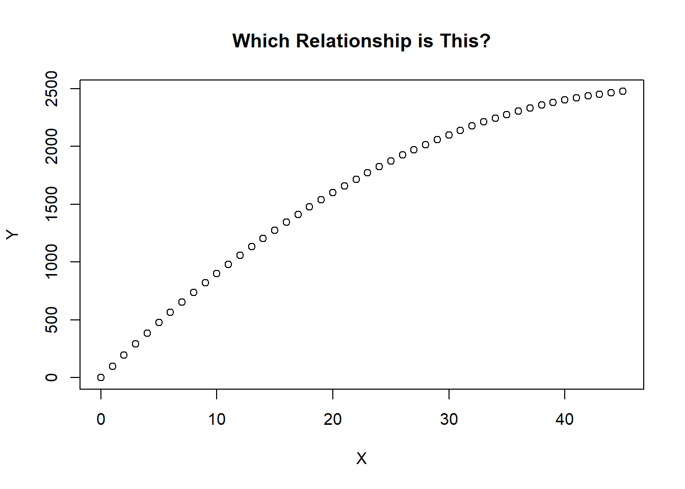
The bottom line is that choosing the wrong non-linear transformation will still lead to some amount of specification bias, but it might not be as much as a linear specification.