11.4 The Quadratic transformation
A quadratic transformation is used when the relationship between a dependent and independent variable changes direction. The slope can start off positive and become negative (the blue line in the figure), or begin negative and become positive (the red line).
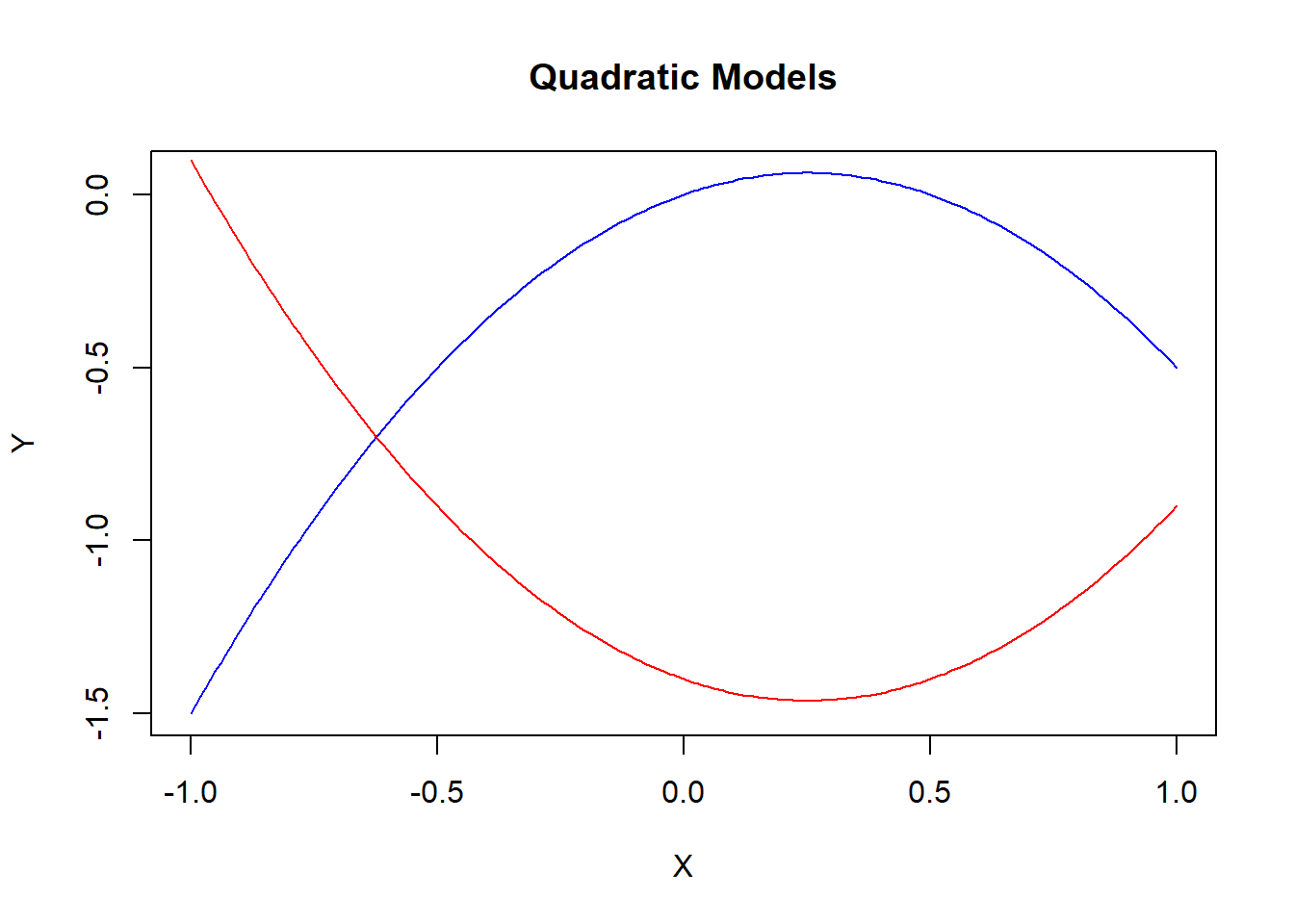
Quadratic models are designed to handle functions featuring slopes that change qualitatively.
\[Y_i = \beta_0 + \beta_1 X_i + \beta_2 X_i^2 + \varepsilon_i\]
Notice that this regression has one variable showing up twice: once linearly and once squared. The regression is still linear in the coefficients, so we can estimate this regression as if the regression contained any two independent variables of interest. In particular, if you defined a new variable \(X_{2i} = X_i^2\), then the model would look like a standard multiple regression.
Once the estimated coefficients are obtained, they are combined to calculate one non-linear slope equation.
\[\frac{\Delta Y}{\Delta X} = \beta_1 + 2\beta_2 X\]
A few things to note about this slope equation.
It is a function of X - meaning that you need to choose a value of the independent variable to calculate a numerical slope. This means you are calculating the expected change in Y from a unit increase in X starting from a particular value.
The slope is increasing or decreasing depending on the values of the coefficients and the independent value of X. The coefficients \(\beta_1\) and \(\beta_2\) are usually of opposite sign. Therefore, the slope is negative if \(\beta_1<0\) and X is small so \(\beta_1 + 2\beta_2 X<0\), or positive if \(\beta_1>0\) and X is small so \(\beta_1 + 2\beta_2 X>0\).43
Just as in the log transformation, this quadratic transformation does not need to be done to every independent variable in the regression. Only those that are suspected to have a relationship with the dependent variable that changes direction.44
Application
Consider some simulated data illustrating the relationship between tax rates and the amount of tax revenue collected by the government. One can intuitively imagine that the government will collect zero revenue if they tax income at zero percent. However, they will also collect zero revenue if they tax at 100 percent because nobody will work if their entire income is taxed away. Therefore, there should be a relationship between tax rate and tax revenue that looks something like the figure below.
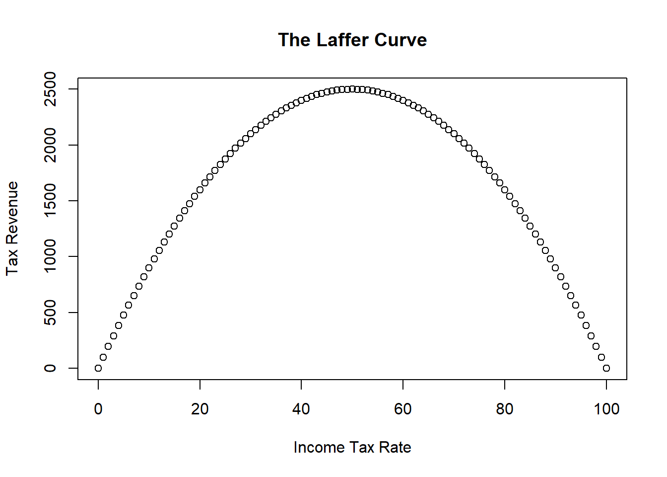
This figure illustrates the infamous Laffer Curve of supply-side economics.45
Suppose you had the data illustrated in the figure. If you assumed a linear relationship between tax revenue and rate, then you will get a very misleading result.
| Estimate | Std. Error | t value | Pr(>|t|) | |
|---|---|---|---|---|
| (Intercept) | 1650 | 151.7 | 10.88 | 1.336e-18 |
| Rate | 2.328e-15 | 2.62 | 8.884e-16 | 1 |
| Observations | Residual Std. Error | \(R^2\) | Adjusted \(R^2\) |
|---|---|---|---|
| 101 | 767.8 | 9.39e-32 | -0.0101 |
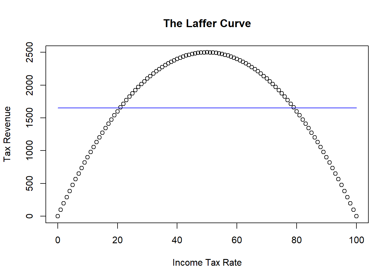
The figure shows that the best fitting straight line is horizontal - meaning that the slope is zero. This linear model would suggest there is no relationship between tax revenue and tax rate. It is partly true - there is just no linear relationship.
| Estimate | Std. Error | t value | Pr(>|t|) | |
|---|---|---|---|---|
| (Intercept) | -7.24e-13 | 2.51e-13 | -2.885 | 0.004818 |
| Rate | 100 | 1.16e-14 | 8.621e+15 | 0 |
| I(Rate^2) | -1 | 1.122e-16 | -8.909e+15 | 0 |
| Observations | Residual Std. Error | \(R^2\) | Adjusted \(R^2\) |
|---|---|---|---|
| 101 | 8.575e-13 | 1 | 1 |
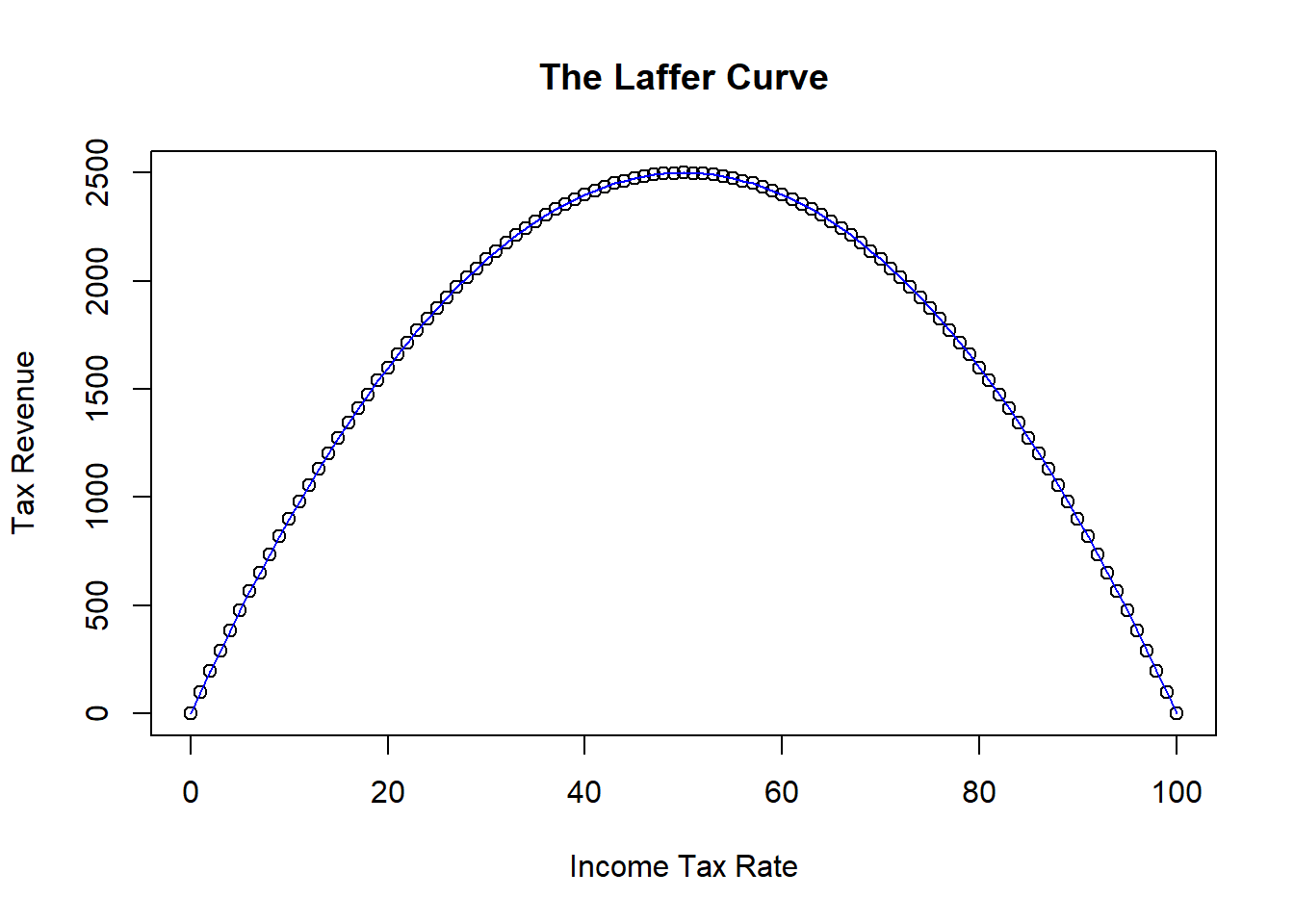
Note that our model has two very statistically significant coefficients and an \(R^2\) of 1. Recall that this data was simulated, so this result isn’t surprising. However, we can now use our results to interpret a non-linear relationship that changes direction as the value of the independent variable gets larger.
\[\frac{\Delta \widehat{Revenue}}{\Delta Rate} = \hat{\beta}_1 + 2\hat{\beta}_2X\]
\[\frac{\Delta \widehat{Revenue}}{\Delta Rate} = 100 + 2(-1)X = 100 - 2X\]
The derivative formula by itself is a bit complicated to interpret on it’s own. One could simply replace the numerical results we have stated in other interpretations with the formula above, but it isn’t terribly informative. One straightforward way of interpreting a nonlinear relationship is to use several values of X to illustrate how the slope changes. Recall that once you plug in a value of X into the slope formula, you are determining what happens when you go from \(X\) to \(X+1\).
\[X = 40 \rightarrow \frac{\Delta \hat{Revenue}}{\Delta Rate} = 20\]
If we plugged in \(X=40\) into our slope equation, we are explicitly determining the expected change in average revenue when the tax rate goes from 40 percent to 41 percent. The answer is 20, meaning that increasing the tax rate to 41 percent will result in an increase in revenue.
\[X = 80 \rightarrow \frac{\Delta \hat{Revenue}}{\Delta Rate} = -60\]
If we plugged in \(X=80\) into our slope equation, we are explicitly determining the expected change in average revenue when the tax rate goes from 80 percent to 81 percent. The answer is -60, meaning that increasing the tax rate to 81 percent will result in a decrease in revenue.
Note that the coefficients do not always need to of opposite sign, because a quadratic is general enough to handle more than a slope that changes direction.↩︎
For example, you will never be able to look at a quadratic transformation for a dummy variable because when the observations are only 0 and 1, then \(X\) and \(X^2\) are technically the same variable!↩︎
We are using this as an example of a quadratic relationship only - I will spare you my tirade on the detrimental use of this (admittedly intuitive) idea by supply-siders.↩︎