11.3 The Log transformation
The natural log transformation is used when the relationship between a dependent and independent variable is not constant in units but constant in percentage changes (or growth rates). Imagine putting $100 in a bank at 5 percent interest. If you kept the entire balance in the account, then after one year you will have $105 (a $5 increase), after two years you will have $110.25 (a $5.25 increase), after three years you will have $115.76 (a $5.76 increase), and so on. What is happening is that the account balance is not growing in constant dollar units, but it is growing in constant percentage units. In fact, the balance is said to be growing exponentially. Things like a country’s output, aggregate prices, and population all grow exponentially because they build on each other just like the compound interest story.
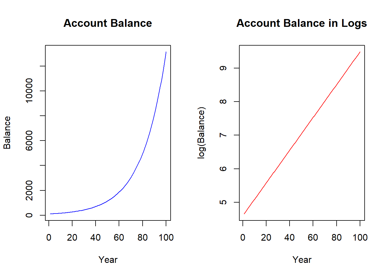
If we kept our $100 dollars in the bank for a very long time, the balance would evolve according to the figure below on the left. The figure illustrates a non-linear relationship between account balance and time - and the slope is getting steeper as time goes on. While we know that the account balance is increasing by larger and larger dollar increments, we also know that it is growing at a constant five percent. We can uncover this constant percentage change by applying the natural log to the balance - as we did to the right figure. You can see that the natural log function straightens the exponential relationship - so the transformed relationship is linear and ready for our regression model.
The derivative of the log function
The natural log function has a very specific and meaningful derivative:
\[\frac{dln(Y)}{dY} = \frac{\Delta Y}{Y}\]
This formula is actually a generalization of the percentage change formula. Suppose you wanted to know the difference between \(Y_2\) and \(Y_1\) in percentage terms relative to \(Y_1\). The answer is
\[\frac{Y_2 - Y_1}{Y_1} * 100\%\]
Therefore, the only thing missing from the log transformation is the multiplication of \(100\%\), which we can do after estimation.
For example, suppose that you didn’t know the average percentage change (or average growth rate) of your account. If Y was your account balance and X was number of years in the account, then you could estimate it. Notice that the slope is approximately 0.05. If you multiply that by \(100\%\) then you have your average interest rate back.
| (Intercept) | X |
|---|---|
| 4.605 | 0.04879 |
Log-log and Semi-log models
Recall that a standard slope is the change in Y over a change in X. Combine this fact with the log of a variable delivers a percentage change in the derivative (provided you multiply by \(100\%\)), and you have several options for which variables you want to consider the logs of. The question you ask yourself is if you want to consider the change of a variable in units or the percentage change of a variable.
Log-log model
A Log-log model is one where both the dependent and the independent variable are logged.
\[ln(Y_i)=\beta_0 + \beta_1 ln(X_i) + \varepsilon_i\]
The slope coefficient \((\beta_1)\) details the percentage change in the dependent variable given a one percent change in the independent variable. To see this, apply the derivative formula above to the entire formula.
\[\frac{dln(Y_i)}{dY} = \beta_1 \frac{dln(X_i)}{dX}\] \[\frac{dln(Y_i)}{dY} * 100\% = \beta_1 \frac{dln(X_i)}{dX} * 100\%\] \[\%\Delta Y_i = \beta_1 \%\Delta X_i\] \[ \beta_1 =\frac{\%\Delta Y_i}{\%\Delta X_i}\]
Semi-log models
Sometimes it makes no sense to take the log of a variable because the percentage change makes no sense. For example, it wouldn’t make sense to take the log of the year in the bank account example above because time is not relative. In other words, a percentage change in time doesn’t make sense. In addition, variables that reach values less than or equal to zero cannot be logged because the natural log is only defined on positive values. In either case, it would make sense to not take the log of some variables.
A Log-lin model is a semi-log model where only the dependent variable is logged. This is like the case with the bank account example above.
\[ln(Y_i)=\beta_0 + \beta_1 X_i + \varepsilon_i\]
\[\frac{dln(Y_i)}{dY} = \beta_1 \Delta X\] \[\frac{dln(Y_i)}{dY} * 100\% = (\beta_1 * 100\%)\Delta X\] \[\frac{\% \Delta Y}{\Delta X}= \beta_1 * 100\%\] Note that the \(100\%\) we baked into the interpretation is explicitly accounted for in order to turn the derivative of the log function into a percentage change.
A Lin-Log model is a semi-log model where only the independent variable is logged. This might come in handy when you want to determine the average change in the dependent variable in response to a percentage-change in the independent variable.
\[Y_i=\beta_0 + \beta_1 ln(X_i) + \varepsilon_i\]
\[\Delta Y=\beta_1 \frac{dln(X_i)}{X_i}\] \[\Delta Y=\beta_1 \frac{dln(X_i)}{X_i}*\frac{100}{100}\] \[\Delta Y=\frac{\beta_1}{100} \%\Delta X\]
\[\frac{\Delta Y}{\%\Delta X}=\frac{\beta_1}{100} \] Note that the derivation for the lin-log model suggests that you must divide the estimated coefficient by 100 in order to state the expected change in the dependent variable due to a percentage change in the independent variable.
It isn’t ALL OR NOTHING!!!
To be clear, if you have a multiple regression model with several independent variables, you get to treat each independent variable however you wish. In other words, if you log one independent variable, you do not need to automatically log the others. This is especially the case when some can be logged while others cannot. The bottom line is that if you have one of the relationships detailed above with the dependent variable and a single independent variable, then you use the correct derivative form and provide the correct interpretation.
In particular, suppose you had the following model
\[ln(Y_i)=\beta_0 + \beta_1 X_{1i} + \beta_2 ln(X_{2i}) + \varepsilon_i\]
This model is a combination between a log-lin model (with respect to \(X_{1i}\)) and a log-log model (with respect to \(X_{2i}\)). The derivatives are therefore
\[\beta_1 * 100\% = \frac{\% \Delta Y}{\Delta X_1}\]
\[\beta_2= \frac{\% \Delta Y}{\%\Delta X_2}\]
Application
If we ran a regression with hourly wage as the dependent variable and tenure (i.e., years on the job) as the independent variable, then we are estimating the average change in dollars for an additional year of tenure. However, it might be more worthwhile to consider an annual average percentage change in wage as opposed to a dollar change. That is what happens for most people, anyway.
| Estimate | Std. Error | t value | Pr(>|t|) | |
|---|---|---|---|---|
| (Intercept) | 1.501 | 0.02687 | 55.87 | 7.261e-223 |
| tenure | 0.02395 | 0.003039 | 7.881 | 1.89e-14 |
| Observations | Residual Std. Error | \(R^2\) | Adjusted \(R^2\) |
|---|---|---|---|
| 526 | 0.5031 | 0.106 | 0.1043 |
The slope estimate gets multiplied by \(100\%\) so we can state that wages increase by \(2\%\) on average for every additional year of tenure.