1.3 Descriptive Measures
This section summarizes the measures we use to describe data samples.
Central Tendency: the central value of a data set
Variation: the dispersion (scattering) around a central value
Shape: the distribution pattern of the data values
These measures will be used repeatedly in our analyses, and will affect how confident we are in our conclusions.
To introduce you to some numerical results in R, we will continue with our light bulb scenario and add some actual data. Suppose we randomly selected 60 light bulbs from our population (i.e., our sample), turned them on, and timed each one until it burned out. If we recorded the lifetime of each light bulb, then we have a dataset (or data sample) of 60 observations on the lifetime of a light bulb. This is what we will be using below.
1.3.1 Central Tendency
The Arithmetic or sample mean is the average value of a variable within the sample.
\[\bar{X}=\frac{\text{Sum of values}}{\text{Number of observations}}=\frac{1}{n} \sum\limits_{i=1}^n X_i\]
# the mean of our light bulb sample:
# First we create a vector containing 60 observations of the lifespan of each of our light bulbs in the sample. The variable is called "Lifetime".

Lifetime=c(858.9164,  797.2652, 1013.5366, 1064.8195,  874.2275,  825.1137,
           897.0879,  924.0998,  870.0674,  966.2095,  955.1281,  977.2073,
           888.1690,  826.6483,  776.7479,  877.5691,  998.7101,  892.8178,
           886.0261,  831.7615, 1082.9650, 1034.9549,  784.5026,  919.2082,
           1049.1824,  923.5767,  907.7295,  890.3758,  856.4240,  808.8035,
           1009.7146,  890.3709,  930.9597,  809.9274,  919.9381,  793.7455,
           919.9824,  948.8593,  810.6887,  846.9573,  955.3873,  833.2762,
           892.4969,  973.1861,  913.7650,  928.6057,  940.7637,  964.4341,
           914.2733,  880.3329,  831.5395,  967.2442, 1030.7598,  857.5421,
           889.3689, 1094.1440,  927.7684,  730.9976,  918.8359,  867.5931)

# Calculate the mean of the variable Lifetime
(mean(Lifetime))
## [1] 907.5552The average lifetime of our 60 \((n=60)\) observed light bulbs is 908 hours.
The median is the middle value of an ordered data set.
If there is an odd number of values in a data set, the median is the middle value
If there an even number, median is the average of the two middle values
## [1] 902.4087The median lifetime of our 60 observed light bulbs is 902 hours.
Percentiles break the ordered values of a sample into proportions (i.e., percentages of the group of individual observations).
Quartiles split the data into 4 equal parts - with each group containing 25 percent of the observations.
Deciles split the data into 10 equal parts - with each group containing 10 percent of the observations.
In general, the pth percentile is given by: \((p * 100)^{th}=p(n+1)\)
A percentile delivers an observed value such that a determined proportion of observations are less than or equal to that value. You can choose any percentile value you wish. For example, the code below calculates the 4th, 40th, 50th, and 80th percentiles of our light bulb sample.
# You can generate any percentile (e.g. the 4th, 40th, 50th, and 80th) using the quantile function:
(quantile(Lifetime,c(0.04, 0.40, 0.50, 0.80)))
## 4% 40% 50% 80%
## 787.8300 888.8889 902.4087 966.4164This result states that 4% of our observations are less that 788 hours, 40% of our observations are less than 889 hours, and 80% of our observations are less than 966 hours. Note that the median (being the middle-ranked observation) is by default the 50th percentile.
##      50%
## 902.4087
The main items of central tendency can be laid out in a Six-Number Summary. This summary delivers the range of our observations (the maximum observed value minus the minimum), the mean, as well as the quartiles of the observations.
- Minimum
- First Quartile (25th percentile)
- Second Quartile (median)
- Mean
- Third Quartile (75th percentile)
- Maximum
##    Min. 1st Qu.  Median    Mean 3rd Qu.    Max.
##   731.0   857.3   902.4   907.6   955.2  1094.1
1.3.2 Variation
The sample variance measures the average (squared) amount of dispersion each individual observation has around the sample mean.
Dispersion is a very important concept in statistics, so take some time to understand exactly what this equation of variation is calculating. In particular, \(X\) represents a variable and \(X_i\) is a single observation of that variable from a sample. Once the mean \((\bar{X})\) is calculated, \(X_i - \bar{X}\) is the difference between a single observation of X and the overall mean of X. Sometimes this difference is negative \((X_i < \bar{X})\) and sometimes this difference is positive \((X_i > \bar{X})\) - which is why we must square these differences before adding them all up. Nonetheless, once we obtain the average value of these differences, we get a sense of how these individual observations are scattered around the sample average. This measure of dispersion is relative. If this value was zero, then every observation of \(X\) is equal to \(\bar{X}\). The greater the value is from zero, the greater the average dispersion of individual values around the mean.
\[S^2=\frac{1}{n-1}\sum\limits_{i=1}^n(X_i-\bar{X})^2\]
The sample standard deviation is the square-root of the sample variance and measures the average amount of dispersion in the same units as the mean. This is done to back-out the fact that we had to square the differences of \(X_i - \bar{X}\), so the variance is technically denoted in squared units.
\[S=\sqrt{S^2}\]
## [1] 6235.852## [1] 78.96741The variance of our sample of light bulb lifetimes is 6236 squared-hours. After taking the square root of this number, we can conclude that the standard deviation of our sample is 79 hours. Is this standard deviation big or small? The answer to this comes when we get to statistical inference.
Discussion
The term \((X_i-\bar{X})\) is squared because individual observations are either above or below the mean. If you don’t square the terms (making the negative numbers positive) then they will sum to zero by design.
The term \((n-1)\) appears in the denominator because this is a sample variance and not a population variance. In a population variance equation, \((n-1)\) gets replaced with \(n\) because we know the population mean. Since we had to estimate the population mean (i.e., used the sample mean), we had to deduct one degree of freedom. We will talk more about degrees of freedom later, but the rule of thumb is that we deduct a degree of freedom every time we build a sample statistic (like sample variance) using another sample statistic (like sample mean).
The coefficient of variation is a relative measure which denotes the amount of scatter in the data relative to the mean.
The coefficient of variation (or CV) is useful when comparing data on variables measured in different units or scales (because the CV reduces everything to percentages).
\[CV=\frac{S}{\bar{X}}*100\%\]
Take for example the Gross Domestic Product (i.e., output) for the states of California and Delaware.
CGDP <- c(1379722, 1470543, 1583231, 1709491, 1707065, 1747200, 1829297,
          1902550, 1988737, 2072274, 2103015, 2110596, 2025633, 2056990,
          2090837, 2144090, 2219611, 2316331, 2437367, 2519134, 2628315,
          2708967, 2800505, 2722839)

DGDP <- c(33400.0, 37065.1, 40427.3, 43515.9, 46555.9, 45828.2, 47731.3,
          51337.7, 52028.2, 54956.7, 56281.3, 54777.6, 57267.3, 57986.7,
          60821.8, 61866.7, 61007.5, 67549.8, 71547.8, 69284.2, 69899.4,
          74186.7, 77082.4, 75512.5)

(mean(CGDP))
## [1] 2094764## [1] 397103.9## [1] 56996.58## [1] 12395.78A quick analysis of the real annual output observations from these two states between the years 1997 and 2020 suggest that the average annual output of California is 2,094,764 million dollars (with a standard deviation of 397,104 million) and that of Delaware is 56,997 million dollars (with a standard deviation of 12,396 million). These two states have lots of differences between them, and it is difficult to tell which state has more volatility in their output.
If we construct coefficients of variation:
## [1] 18.95698## [1] 21.74828We can now conclude that Delaware’s standard deviation of output is almost 22% that of its’ average output, while California’s standard deviation is 19%. This would suggest that Delaware has the more volatile output, relatively speaking, but they aren’t that different.
1.3.3 Measures of shape
A distribution is a visual representation of a group of observations. We are going to be looking at plenty of distributions in the following chapters, so it will help to get an idea of their characteristics.
Comparing the mean and median of a sample will inform us of the skewness of the distribution.
- mean = median: a symmetric or zero-skewed distribution.
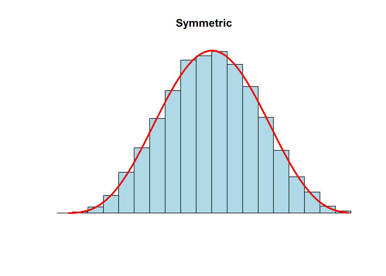
mean > median: a positive-skewed or right-skewed distribution
- the right-tail is pulled in the positive direction
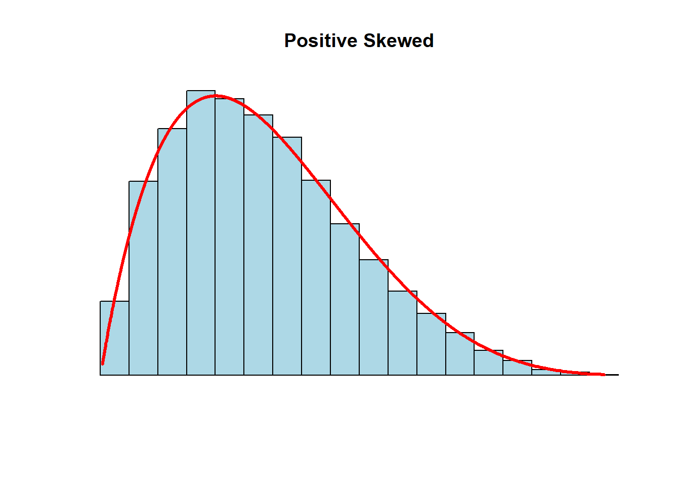
mean < median: a negative-skewed or a left-skewed distribution
- the left-tail is pulled in the negative direction
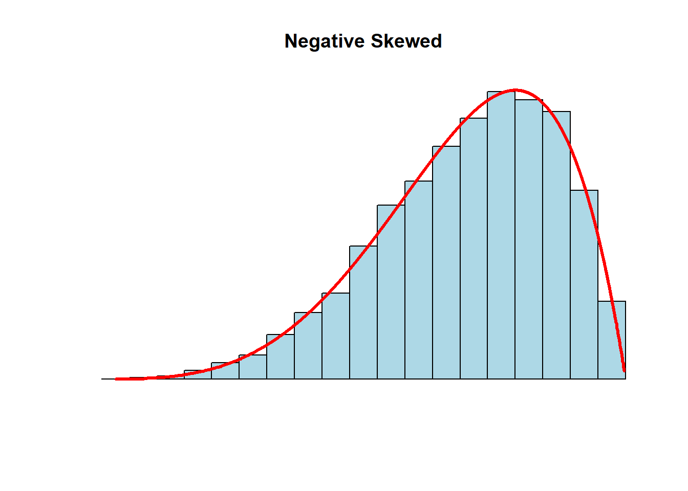
The degree of skewness is indicative of outliers (extreme high or low values) which change the shape of a distribution.
A classic economic example of a positive-skewed distribution is the average income distribution in the US. A large proportion of the individuals fall in the either the low-income or middle-income brackets, with a very small proportion falling in the high-income bracket. This high-income group pulls up the average amount of individual average income, but doesn’t impact the median income because they are not in the bottom 50%. This is why mean > median in that distribution.
1.3.4 Covariance and Correlation
We won’t be examining relationships between different variables (i.e., multivariate analyses) until later on in the companion, but we can easily calculate and visualize these relationships.
The covariance measures the strength of the relationship between two variables. This measure is similar to a variance, but it measures how the dispersion of one variable around its mean varies systematically with the dispersion of another variable around its mean. The covariance can be either positive or negative (or zero) depending on how the two variables move in relation to each other.
\[cov(X,Y)=\frac{1}{n-1}\sum\limits_{i=1}^n(X_i-\bar{X})(Y_i-\bar{Y})\]
The coefficient of correlation transforms the covariance into a relative measure.
\[corr(X,Y)=\frac{cov(X,Y)}{S_{X}S_{Y}}\] The correlation transformed the covariance relationship into a measure between -1 and 1.
\(corr(X,Y)=0\): There is no relationship between \(X\) and \(Y\). This corresponds to a covariance of zero.
\(corr(X,Y)>0\): There is a positive relationship between \(X\) and \(Y\) - meaning that the two variables tend to move in the same direction. This corresponds to a large positive covariance.
\(corr(X,Y)<0\): There is a negative relationship between \(X\) and \(Y\) - meaning that the two variables tend to move in the opposite direction. This corresponds to a large negative covariance.
Extended Example:
This chapter concludes with a summary of all of the descriptive measures we discussed. Consider a dataset that is internal to R (called mtcars) that contains characteristics of 32 different automobiles. We will focus on two variables: the average miles per gallon (mpg) and the weight of the car (in thousands of pounds).
car <- mtcars # This command loads the dataset and calls it car

# Lets examine mpg first:
summary(car$mpg)
## Min. 1st Qu. Median Mean 3rd Qu. Max.
## 10.40 15.43 19.20 20.09 22.80 33.90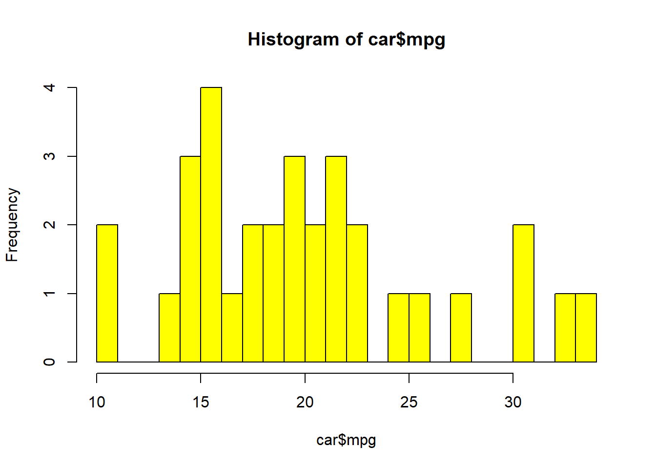
## [1] 36.3241## [1] 6.026948The above analysis indicates the following:
The sample average MPG in the sample is 20.09, while the median in 19.20. This indicates that there is a slight positive skew to the distribution of observations.
The lowest MPG is 10.4 while the highest is 33.90.
The first quartile is 15.43 while the third is 22.80. This delivers the inter-quartile range (the middle 50% of the distribution)
The standard deviation is 6.03 which delivers a 30 percent coefficient of correlation.
##    Min. 1st Qu.  Median    Mean 3rd Qu.    Max.
##   1.513   2.581   3.325   3.217   3.610   5.424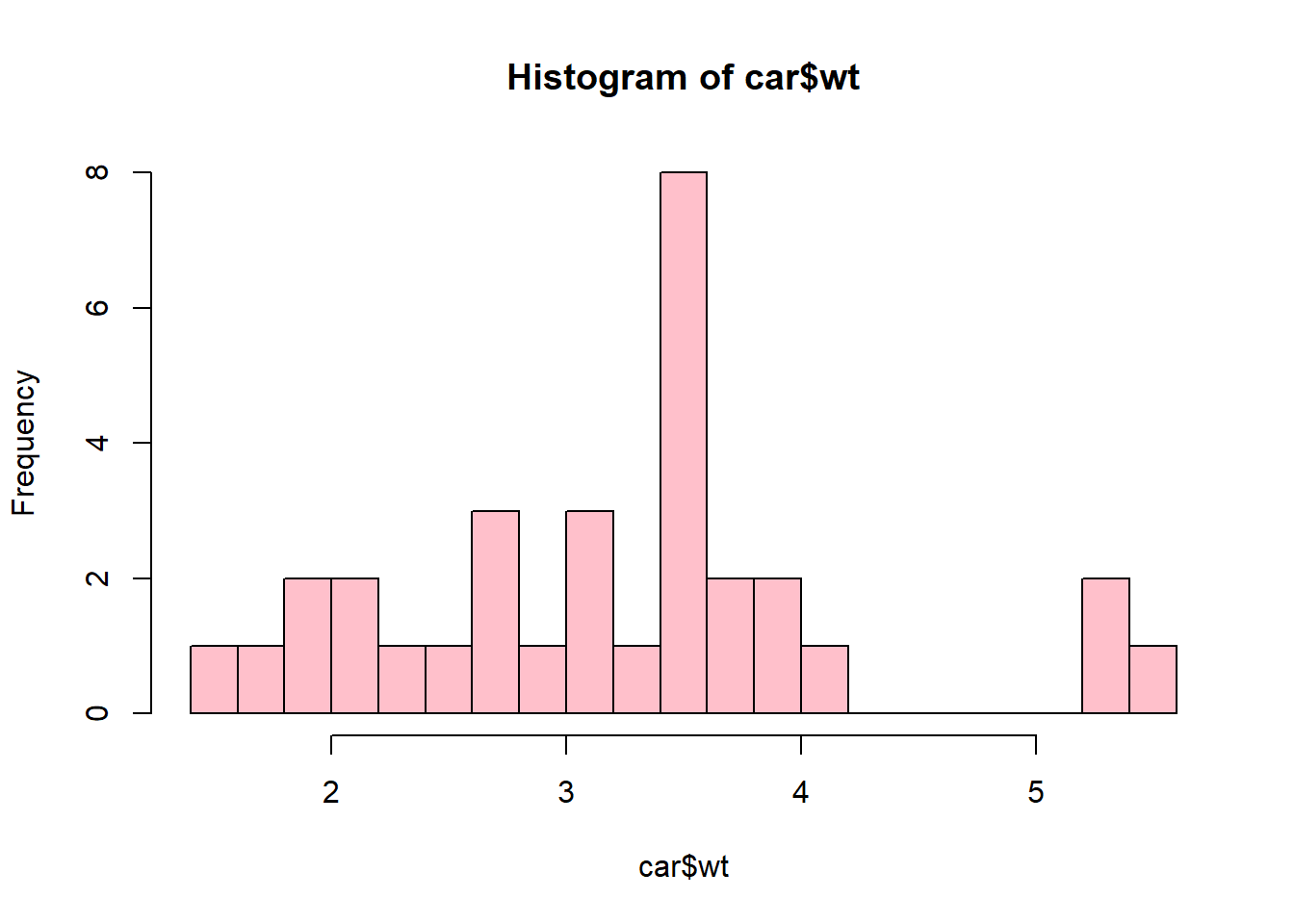
## [1] 0.957379## [1] 0.9784574The above analysis indicates the following:
The sample average weight in the sample is 3.22 thousand pounds, while the median in 3.33. This indicates that there is a slight negative skew to the distribution of observations.
The lowest weight is 1.51 while the highest is 5.42.
The first quartile is 2.58 while the third is 3.61.
The standard deviation is 0.99 which also delivers a 30 percent coefficient of correlation.
## [1] -5.116685## [1] -0.8676594plot(car$mpg,car$wt, pch=16,
xlab = "Miles per gallon",
ylab = "Weight of car",
main = "A Scatter plot",
col = "cyan")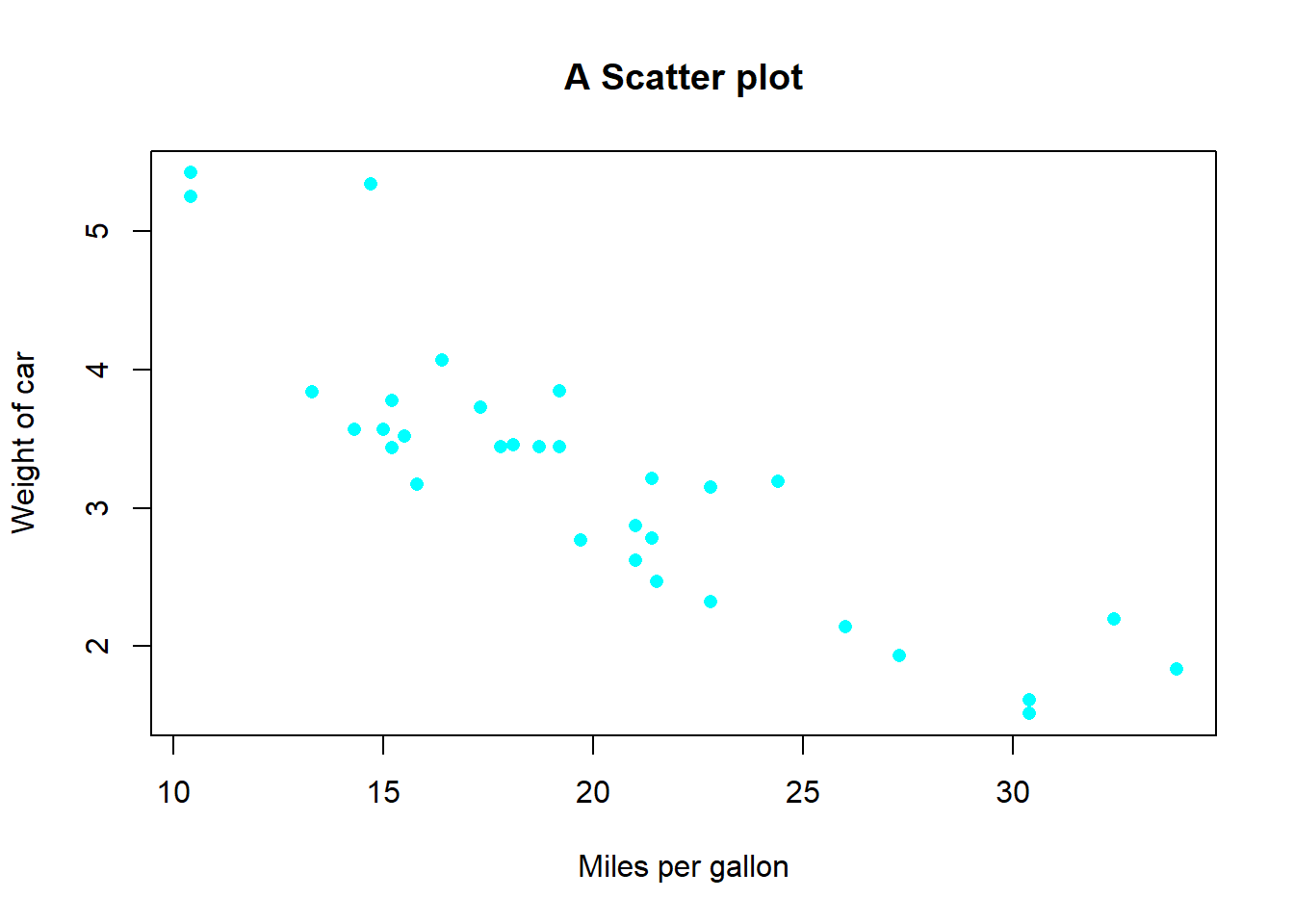
The negative correlation as well as the obviously negative relationship in the scatter-plot between the weight of a car and its miles per gallon should make intuitive sense - heavy cars are less efficient.
The Punchline
Suppose we want to learn about a relationship between a car’s weight and its fuel efficiency. Our sample is 32 automobiles, but our population is EVERY automobile (EVER).1 We would like to say something about the population mean Weight and MPG.
How does the sample variance(s) give us confidence on making statements about the population mean when we’re only given the sample? That’s where inferential statistics comes in. Before we get into that, we will dig into elements of collecting data (upon which our descriptive statistics are based on) and using R (with which we will use to calculate our descriptive statistics using our collected data).
We could add more criteria such as every sedan, with a six-cylinder engine, etc.↩︎