11.5 The Reciprocal transformation

Suppose a relationship doesn’t change directions as much as it dies out.

\[Y_i = \beta_0 + \beta_1 \frac{1}{X_i} + \varepsilon_i\]

As in the quadratic transformation, this model is easily estimated by redefining variables (i.e., \(X_{2i}=1/X_i\)). The slope of this function can be obtained using our standard derivative function and noting that \(1/X_i = X_i^{-1}\)

\[Y_i = \beta_0 + \beta_1 \frac{1}{X_i} + \varepsilon_i\] \[Y_i = \beta_0 + \beta_1 X_i^{-1} + \varepsilon_i\] \[\frac{\Delta Y}{\Delta X} = -\beta_1 X_i^{-2}=\frac{-\beta_1} {X_i^{2}}\]

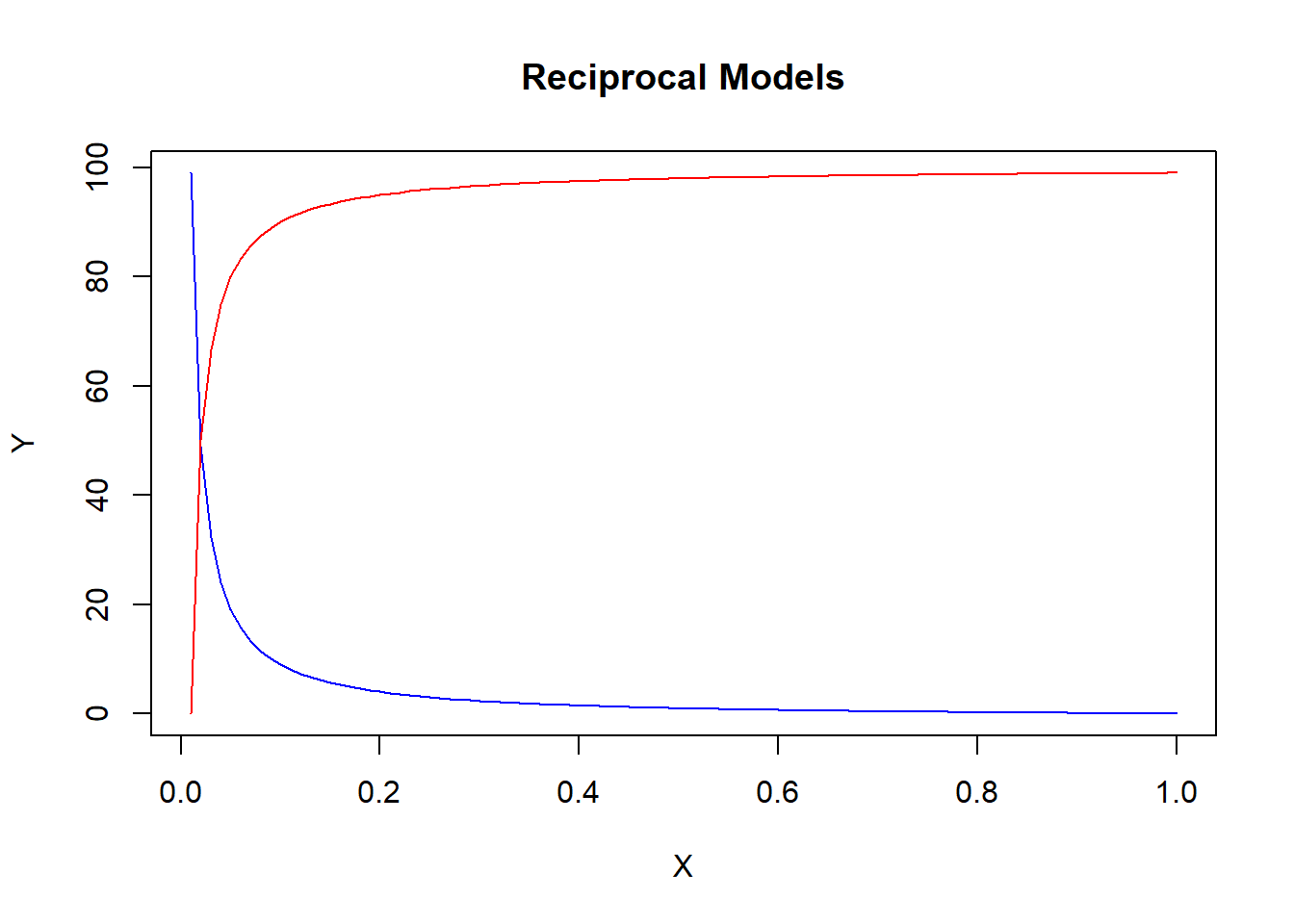
Notice again that a value of the independent variable is needed to calculate the slope of the function at a specific point. However, as X gets larger, the slope approaches zero. A slope of zero is a horizontal line - and that is when the relationship between Y and X dies out. If \(\beta_1>0\) then the slope begins negative and approaches zero from above (the blue line). If \(\beta_1<0\) then the slope begins positive and approaches zero from below (the red line).

Application

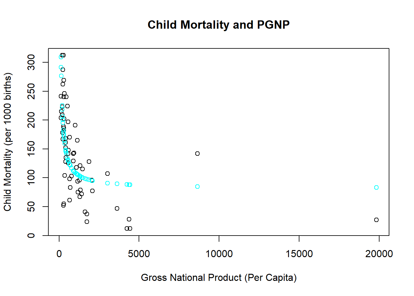
The richer a nation is, the better a nation’s health services are. However, a nation can eventually get to a point that health outcomes cannot improve no matter how rich it gets. This application considers child mortality rates of developing and developed countries and uses the wealth of a country measured by per-capita gross national product (PGNP) to help explain why the child mortality rate is different across countries.

library(readxl)
CM <- read_excel("data/CM.xlsx")

REG <- lm(CM$CM ~ I(1/CM$PGNP))

	Estimate	Std. Error	t value	Pr(>|t|)
(Intercept)	81.79	10.83	7.551	2.38e-10
I(1/CM$PGNP)	27273	3760	7.254	7.821e-10

Fitting linear model: CM\(CM ~ I(1/CM\)PGNP)

Observations	Residual Std. Error	\(R^2\)	Adjusted \(R^2\)
64	56.33	0.4591	0.4503

The estimated coefficient is large and positive. However, this isn’t the entire slope, because you need to consider the derivative formula above.

\[\frac{\Delta Y}{\Delta X} = \frac{-27,273} {X_i^{2}}\]

If you wanted to consider the impact on child mortality of making a relatively poor nation richer, you plug a low value for PGNP like 100. If you want to consider a richer nation, consider a larger value like 1000.

\[\frac{\Delta Y}{\Delta X} = \frac{-27,273} {100^{2}} = -2.73\] \[\frac{\Delta Y}{\Delta X} = \frac{-27,273} {1000^{2}} = -0.0273\] These calculations show that increasing the wealth of richer countries has a smaller impact on child mortality rates. This should make sense, and it takes a reciprocal model to capture it.