3.5 Coding Basics
Now that your software is ready to go, this section introduces you to how R likes to be talked to. Note that the subsequent chapters are full of commands that you will need to learn when the time comes. In the meantime, here are just a few general pointers.
R is what is known as a line command computing language - meaning that it doesn’t need to compile code prior to execution. That being said, try the following command at the prompt in your console (>):
## [1] 16See? Just a big calculator.
3.5.1 Installing Packages
In order for R to be able to do some of the sophisticated things we will be doing in the course, we need to install source code called packages.
Whenever you need a package, all you need to do is type:
install.packages("name of package")Once this is done, the package is installed in your version of R and you will never need to install it again.9 You will need to unpack the packages each time you want to use them by calling a library command, but we will get to that later.
The first R-script you will create and run as part of your first assignment contains an executable portion of the code looks like this:
install.packages( c("AER", "car", "dplyr",
"fastDummies", "readxl", "xtable", "vars",
"WDI", "xts", "zoo", "wooldridge") )
This is a simple command that asks R to download 11 packages and install them. You can easily make your own RScript by opening up a blank RScript in R, and copying the code in the gray box above.10 Highlight the portion above in your RScript, and hit the Run tab at the top of the upper-left window of RStudio. A bunch of notifications will appear on the R console (lower-left window) while the list of packages will be downloaded from the mirror site you selected earlier and installed. This can take some time (about 20 mins) depending on your internet connection, so it is advised you do this when you can leave your computer alone for awhile.
3.5.2 Assigning Objects
We declare variable names and other data objects by assigning names. For example, we can repeat the calculation above by first assigning some variables:
## [1] 16Notice that all of these variable names should now be in your global environment (upper-right window). The reason why 16 was returned on the console is because we put the last command in parentheses. That is, parentheses around a calculation is considered the print to screen command.
You might be asking why R simply doesn’t use an equal sign in stead of the assign sign. The answer is that we will be assigning names to output objects that contain much more than a single number. Things like regression output is technically assigned a name, so we are simply being consistent. You can use an equal sign in place of the assign sign for some cases, and everything will go through equally well. However, this doesn’t work for every command we will use in this class.
3.5.3 Listing, Adding, and Removing
We can list all objects in our global environment using the list command: ls()
##  [1] "alpha"       "BIG"         "car"         "CGDP"        "df"
##  [6] "DGDP"        "i"           "i1"          "i2"          "left"
## [11] "Lifetime"    "mu"          "n"           "N"           "probability"
## [16] "Pval"        "right"       "S"           "Sig"         "SMALL"
## [21] "t"           "t_values"    "tcrit"       "TOTAL"       "x"
## [26] "X"           "Xbar"        "xtick"       "Y"           "Zstat"
As we already showed, we can add new variables by simply assigning names to our calculations.
If you ever wanted to remove some variables from your global environment, you can use the remove command: rm(name of variable)
3.5.4 Importing Data
R can handle data in almost any format imaginable. The main data format we will consider in this class is a trusty old MS Excel file.11 It is recommended that you put all of you data files somewhere easy to access. Like a single folder directly on your C drive.12
There are two ways to import data, and we will go over them in turn. Either one of these way will work as described if you are using installed versions of R and RStudio on your computer. However, if you are using the Posit Cloud, there is one small initial step.
POSIT CLOUD USERS
Before importing any data into R, you must first upload the data onto your portion of the cloud server. This can be done by selecting the Upload button in the lower-right portion of the screen (see enlarged image below). Selecting the upload button will open a window where you can select the data file from your computer, which will then be added to your server account. Once the data is there, you can proceed with the steps below.
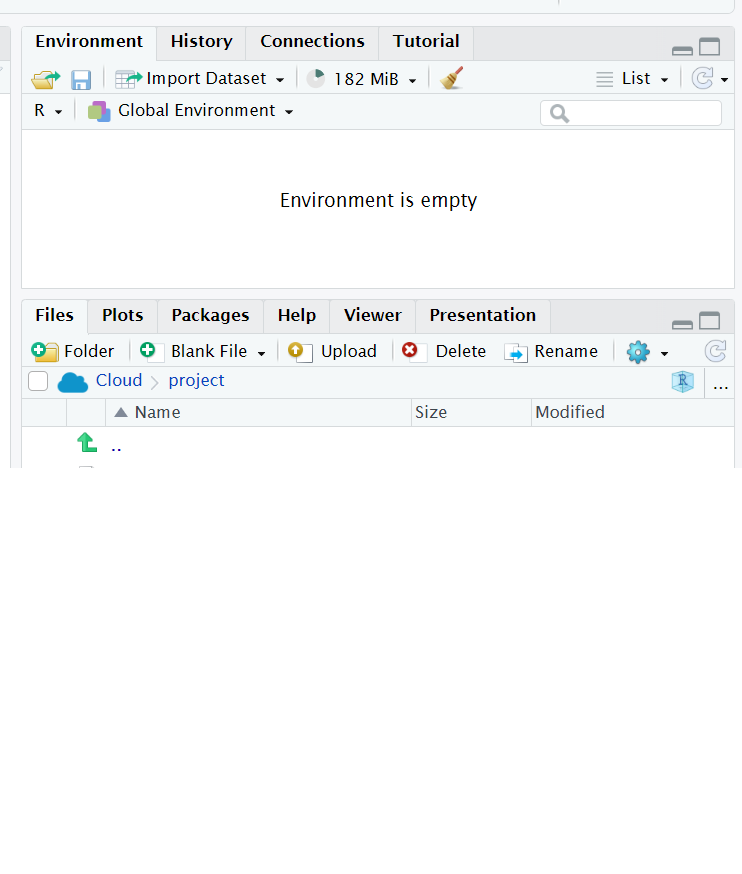
Figure 3.5: Uploading files to the Server
1. The Direct Way
Once you locate a data file on your computer, you can direct R to import the file and assign it any name you want. The example below imports a dataset of automobile sales called AUTO_SA.xlsx and names it CARDATA.
The term “data/AUTO_SA.xlsx” is the exact location on my computer for this data file. Once you change the file path to your specification… you’re done!
2. The Indirect (but easy) Way
You can also import data directly into R through Rstudio.
Use the files tab (bottom-right window of your screen) and locate the data file you want to import.13
Left-click on file and select Import Dataset…
The import window opens and previews your data.
If everything looks good, hit Import and your done.
Note that the import window in step 3 has a code preview section which is actually writing the code needed to import the dataset. It will look exactly like what your code would need to look like in order to import data the direct way. You can refer to that for future reference.
3.5.5 Manipulating Data
You should now have a dataset named CARDATA imported into your global environment. You can examine the names of the variables inside the dataset using the list command - only this time we reference the name of the dataset.
## [1] "AUTOSALE" "CPI" "DATE" "INDEX" "MONTH" "YEAR"When referencing a variable within a dataset, you must reference both the names of the dataset and variable so R knows where to get it. The syntax is:
Dataset$Variable
For example, if we reference the variable AUTOSALE by stating that it is in the CARDATA dataset.
CARDATA$AUTOSALE
We can now manipulate and store variables within the dataset by creating variables for what ever we need. For example, we can create a variable for real auto sales by dividing autosales by the consumer price index (CPI).
## [1] "AUTOSALE" "CPI"      "DATE"     "INDEX"    "MONTH"    "RSALES"
## [7] "YEAR"
3.5.6 Subsetting Data
Sometimes our dataset will contain more information than we need. Let us narrow down our dataset to see how we can get rid of unwanted data. You should see a little Excel looking icon to the left of the name CARDATA up in the global environment window. If you click on it, you should see the following:
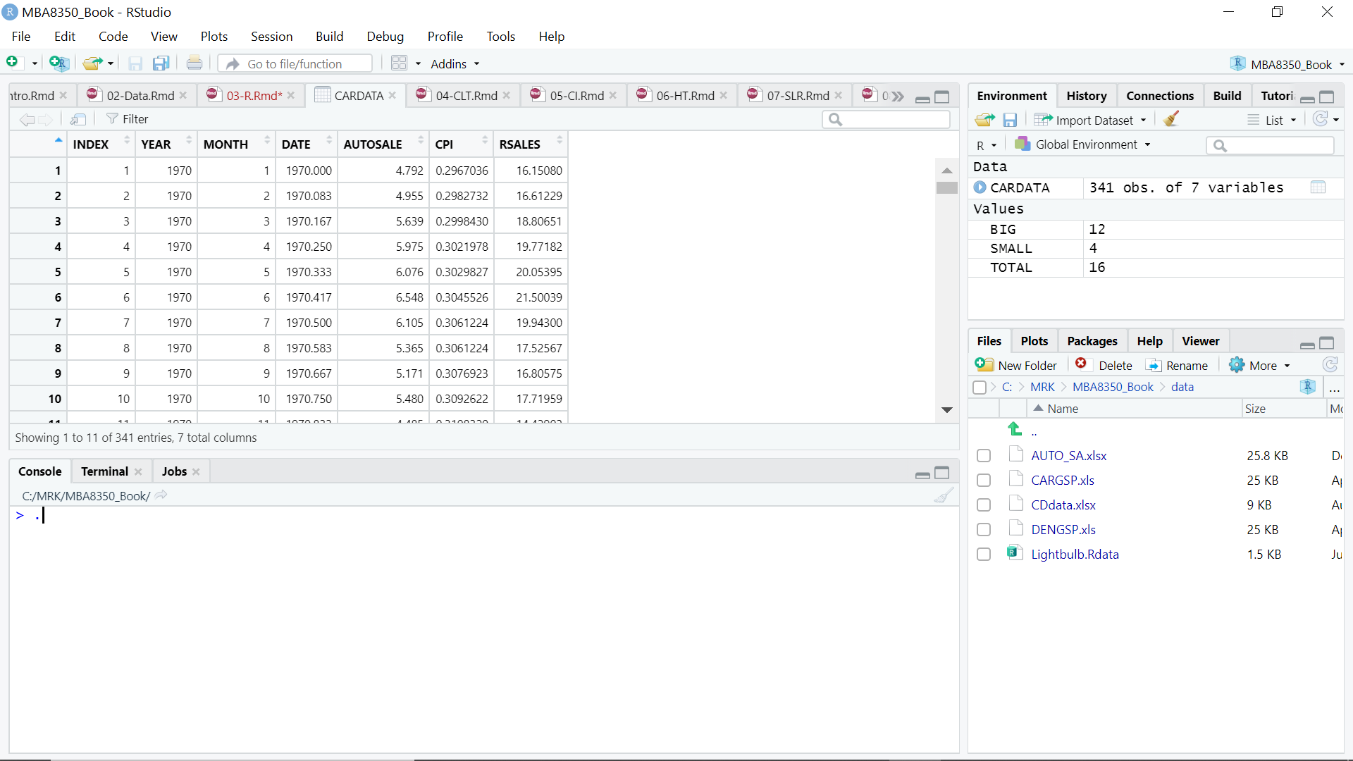
Figure 3.6: A Dataset in R
Thinking of the data set as a matrix with 341 rows and 7 columns will help us understand the code needed to select specific portions of this data.
Note that the variable MONTH cycles from 1 to 12 indicating the months of the year. Suppose we only want to analyze the 12th month of each year (i.e., December). We can do this by creating a new dataset that keeps only the rows associated with the 12 month.
What the above code does is treat the dataset CARDATA as a matrix and lists it as [rows,columns]. The rows instruction is to only keep rows where the month is 12. The columns instruction is left blank, because we want to keep all columns.
You need to do this for your Cloud-based version of R as well.↩︎
You can also get the code directly from the first assignment.↩︎
Note that there is a zip file associated with this companion that contains all data files needed for replication. You will need to download that zip file onto your computer and unzip it before proceeding.↩︎
A folder on your desktop is the worst place for a data folder, because the file path is very messy. The closer to the C: drive, the better.↩︎
This can also be done by selecting File in the upper-left of your screen, then Import Dataset, then From Excel….↩︎