5.2 Deriving a Confidence Interval
Recall when we randomly draw a sample from a sampling distribution and use it to calculate a sample mean \((\bar{X})\), we essentially state that a sample mean is a random variable. Since the CLT states that the sampling distribution is a normal distribution, then this further states that the sample mean is a normally distributed random variable with a mean of \(\mu\) and a standard deviation of \(\frac{\sigma}{\sqrt{n}}\).
\[\bar{X} \sim N\left(\mu,\frac{\sigma}{\sqrt{n}}\right)\]
We can apply our standardization trick so we have
\[Z=\frac{\bar{X}-\mu}{(\sigma/\sqrt{n})}\]
Suppose we have a sample of size \(n\), calculated a sample mean \(\bar{X}\), and that we know the population standard deviation \(\sigma\) (more on this later). If we know these values, then we can use the standard normal distribution as well as the normalization above to draw statistical inference on the population parameter \(\mu\).
What can we say about \(\mu\)?
Since our sample has the same characteristics as the population (by design), we would like to say \(\mu = \bar{X}\) (i.e., \(Z=0\)), but this is not likely. Recall the dice example discussed earlier, while 7 (the population mean) is the most likely average of a sample, there is a larger likelihood of a sample average close to, but not exactly equal to the population mean.
Since \(\bar{X}\) is a single draw from a normal distribution, we can construct a probabilistic range around \(\mu\). This range requires an arbitrary level of confidence \((1-\alpha)\) - which provides bounds for the Z distribution (i.e., it gives us the area under the curve).
We therefore start with a probabilistic statement using a standard normal distribution:
\[Pr\left(-Z \leq \frac{\bar{X}-\mu}{(\sigma/\sqrt{n})} \leq Z\right)=1-\alpha\]
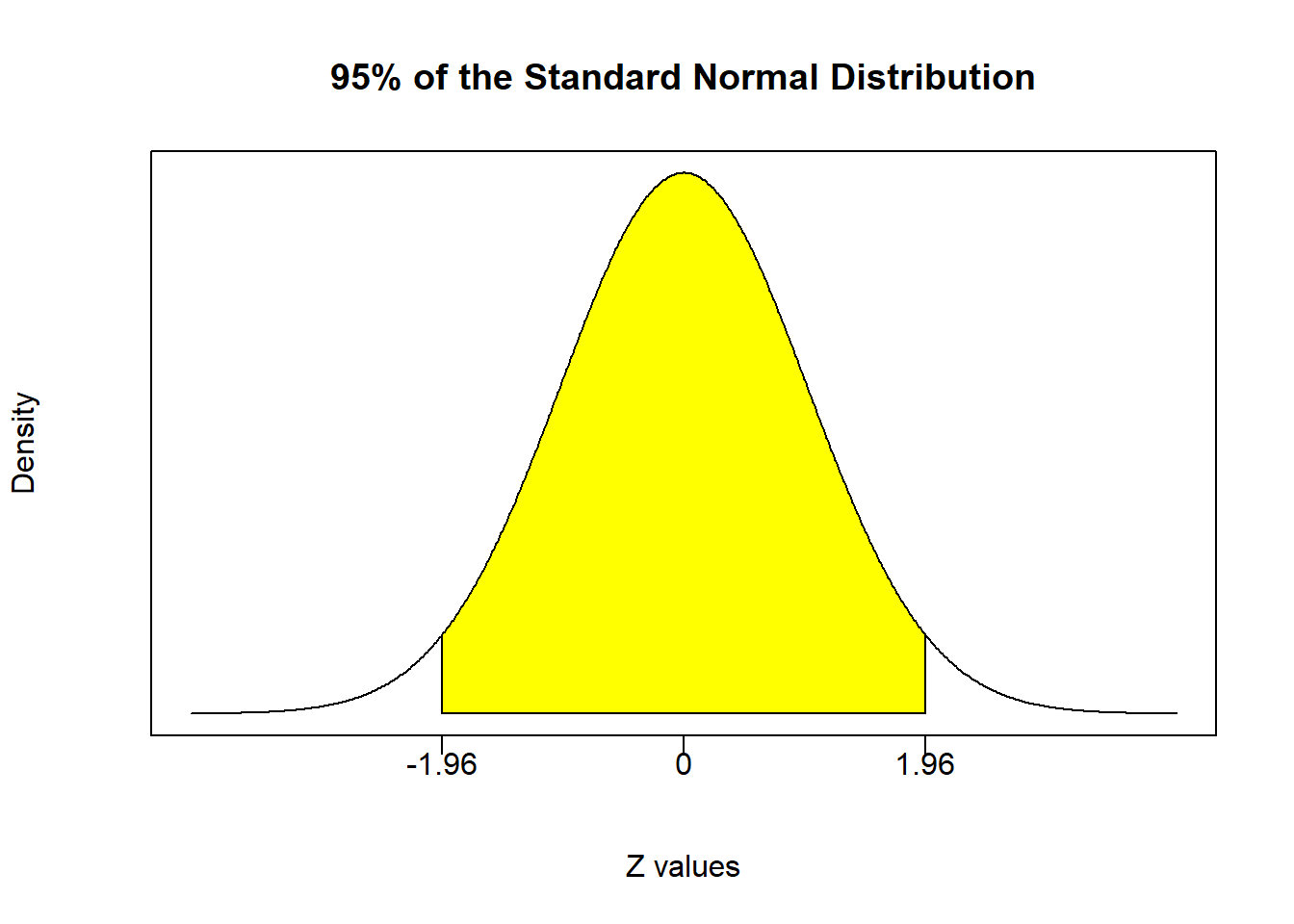
This states (in general terms) that the probability of realizing a value of \(\frac{\bar{X}-\mu}{(\sigma/\sqrt{n})}\) drawn from a standard normal distributed random variable to be between the values -Z and Z is equal to \(1-\alpha\). To put this into context, suppose I set \(\alpha=0.05\) so \(1-\alpha=0.95\) implies that I am looking for something that will occur with 95% probability. Recall the normal distribution has the nice property that 95% of the probability space is between \(1.96\) standard deviations above and below the mean.
Finding these numbers requires another R command: qnorm.
qnorm(p, mean = 0, sd = 1, lower.tail = TRUE)Just like how pnorm takes a quantity and returns a probability, qnorm takes a probability and returns a quantity.
## [1] -1.959964## [1] -1.959964\[Pr\left(-1.96 \leq \frac{\bar{X}-\mu}{(\sigma/\sqrt{n})} \leq 1.96\right)=0.95\]
Now back to our statement for a general \(\alpha\) and \(Z\):
\[Pr\left(-Z \leq \frac{\bar{X}-\mu}{(\sigma/\sqrt{n})} \leq Z\right)=1-\alpha\]
Suppose for the moment that we know the value of \(\sigma\). Given that the only thing we do not know is the other population parameter \(\mu\), we can rearrange the inequalities inside the probability statement to deliver a probabilistic range where we think this parameter will reside.
\[Pr\left(-Z \leq \frac{\bar{X}-\mu}{(\sigma/\sqrt{n})} \leq Z\right)=1-\alpha\]
\[Pr\left(-Z\frac{\sigma}{\sqrt{n}} \leq \bar{X}-\mu \leq Z\frac{\sigma}{\sqrt{n}}\right)=1-\alpha\]
\[Pr\left(-\bar{X}-Z\frac{\sigma}{\sqrt{n}} \leq -\mu \leq -\bar{X}+Z\frac{\sigma}{\sqrt{n}}\right)=1-\alpha\]
\[Pr\left(\bar{X}-Z\frac{\sigma}{\sqrt{n}} \leq \mu \leq \bar{X}+Z\frac{\sigma}{\sqrt{n}}\right)=1-\alpha\]
This statement is a confidence interval, which can be written concisely as
\[\bar{X}-Z_{\frac{\alpha}{2}}\frac{\sigma}{\sqrt{n}} \leq \mu \leq \bar{X}+Z_{\frac{\alpha}{2}}\frac{\sigma}{\sqrt{n}}\]
or
\[\bar{X} \pm Z_{\frac{\alpha}{2}}\frac{\sigma}{\sqrt{n}}\]
It explicitly states that given the characteristics of the sample \((\bar{X},n,\sigma)\) and an arbitrary level of confidence that gives us the probability limits from the standard normal distribution \((Z_{\frac{\sigma}{2}})\), we can build a range of values where we can state with \((1-\alpha) \times 100%\) confidence that the population parameter will reside within.
Welcome to statistical inference!
5.2.1 Application 3
A paper manufacturer produces paper expected to have a mean length of 11 inches, and a known standard deviation of 0.02 inch. A sample of 100 sheets is selected to determine if the production process is still adhering to this length. If it isn’t, then the machine needs to go through the costs of being taken off line and serviced. The sample of 100 sheets was collected and calculated to have an average value of 10.998 inches.
\[\bar{X} = 10.998, \quad n = 100, \quad \sigma = 0.02\]
Construct a 95% confidence interval around the average length of a sheet of paper in the population.
- Since we want 95% confidence, we know that \(\alpha = 0.05\) and we need the critical values from a standard normal distribution such that 95% of the probability distribution is between them. These critical values were calculated previously to -1.96 and 1.96 and are illustrated below. Note that since the shaded region is 95% of the central area of the distribution, we are chopping of 5% of the total area from both tails combined. That means 2.5% is chopped off of each tail.
- Now using the positive critical Z value in our confidence interval equation, we have:
\[\bar{X} \pm Z_{\frac{\alpha}{2}}\frac{\sigma}{\sqrt{n}}\]
\[10.998 \pm 1.96\frac{0.02}{\sqrt{100}}\]
Using R for the calculations:
Xbar = 10.998
n = 100
Sig = 0.02
alpha = 0.05
Z = qnorm(alpha/2,lower.tail = FALSE)
(left = Xbar - Z * Sig / sqrt(n))
## [1] 10.99408## [1] 11.00192\[ 10.99408 \leq \mu \leq 11.00192 \]
Conclusion: I am 95% confident that the mean paper length in the population is somewhere between 10.99408 and 11.00192 inches.
Note that any value within this range is equally likely!
5.2.2 What if we want to change confidence?
If we want to increase the confidence of our statement to 99% or lower it 90%, then we change \(\alpha\) and calculate a new critical Z value. Everything else stays the same.
alpha = 0.01 # increase confidence to 99%
Z = qnorm(alpha/2,lower.tail = FALSE)
(left99 = Xbar - Z * Sig / sqrt(n))
## [1] 10.99285## [1] 11.00315alpha = 0.10 # decrease confidence to 90%
Z = qnorm(alpha/2,lower.tail = FALSE)
(left90 = Xbar - Z * Sig / sqrt(n))## [1] 10.99471## [1] 11.001295.2.3 What happens to the size of the confidence interval when we increase our confidence?
Our three previous conclusions are as follows:
I am 90% confident that the mean paper length in the population is somewhere between 10.9947103 and 11.0012897 inches.
I am 95% confident that the mean paper length in the population is somewhere between 10.9940801 and 11.0019199 inches.
I am 95% confident that the mean paper length in the population is somewhere between 10.9928483 and 11.0031517 inches.
Notice that as our (arbitrary) level of confidence gets larger, the range of our expected population value gets wider. This illustrates a very important distinction in the world of inferential statistics between confidence and precision. If you want me to make a statement with a higher level confidence (i.e., a higher probability of being correct), then I will sacrifice the precision of my answer and simply increase the range of possible values. Suffice it to say, we can increase our confidence up to the point where our confidence interval becomes useless.
\[ Pr(-\infty \leq \mu \leq \infty) = 1.00 \]
I am 100% confident that the mean paper length in the population is somewhere between \(-\infty\) and \(\infty\) inches.