7.6 A Concluding Application
Our course comes with a series of videos that build upon the analysis of a single question: What explains the median starting salary of a class of law students? The code and results will be included at the end of each subsequent chapter in this course companion for comparison purposes.
We start with a very basic theory stating that the median starting salary of a class of law students can be explained by their median LSAT score. Intuitively, a higher median LSAT score suggests that the class is of a higher quality, and therefore should have a higher median starting salary on average. Our Population Regression Function (PRF) is as follows.
\[SALARY_i = \beta_0 + \beta_1 \; LSAT_i + \varepsilon_i\]
library(readxl)
LAW <- read_excel("data/LAW.xlsx")

plot(LAW$LSAT,LAW$SALARY,
     cex = 1,pch=16,col = "blue",
     xlab = "Median LSAT (points)",
     ylab = "Median Starting Salary (dollars)")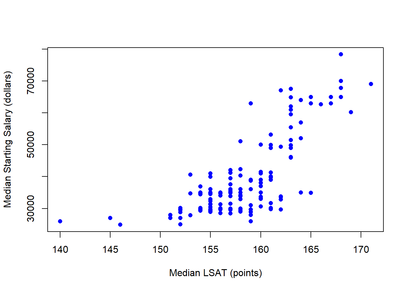
We can use our PRF and the data to arrive at a Sample Regression Function (SRF):
\[SALARY_i = \hat\beta_0 + \hat\beta_1 \; LSAT_i + e_i\]
##
## Call:
## lm(formula = SALARY ~ LSAT, data = LAW)
##
## Residuals:
##      Min       1Q   Median       3Q      Max
## -17188.4  -4801.8   -991.8   4164.9  22531.6
##
## Coefficients:
##              Estimate Std. Error t value Pr(>|t|)
## (Intercept) -267460.1    23210.7  -11.52   <2e-16 ***
## LSAT           1936.7      146.6   13.21   <2e-16 ***
## ---
## Signif. codes:  0 '***' 0.001 '**' 0.01 '*' 0.05 '.' 0.1 ' ' 1
##
## Residual standard error: 8199 on 140 degrees of freedom
## Multiple R-squared:  0.555,  Adjusted R-squared:  0.5519
## F-statistic: 174.6 on 1 and 140 DF,  p-value: < 2.2e-16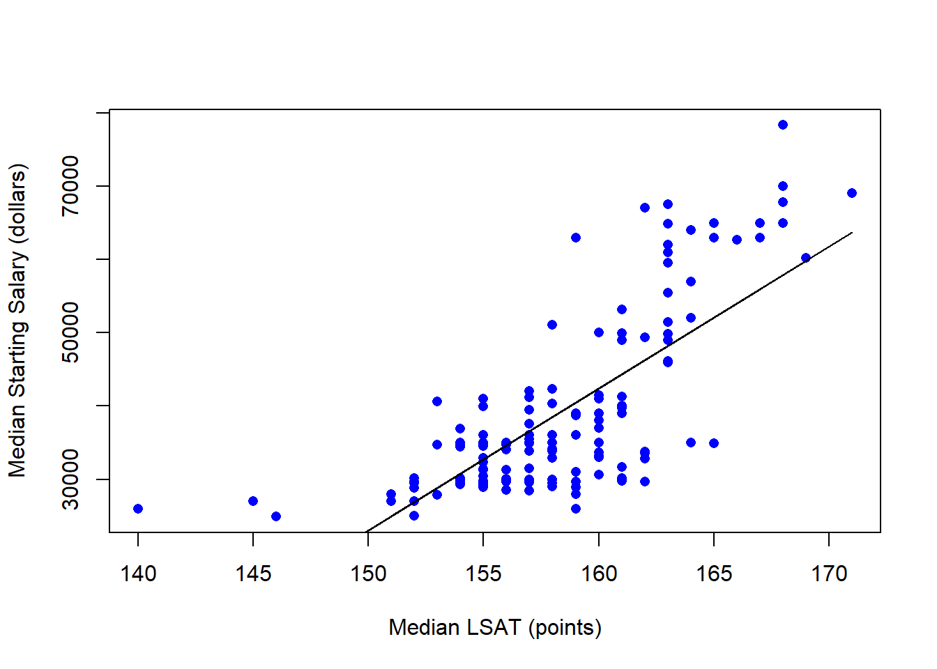
We will hold off on the inferential statistics of this model until next chapter. For now, we can simply interpret the model.
Intercept term
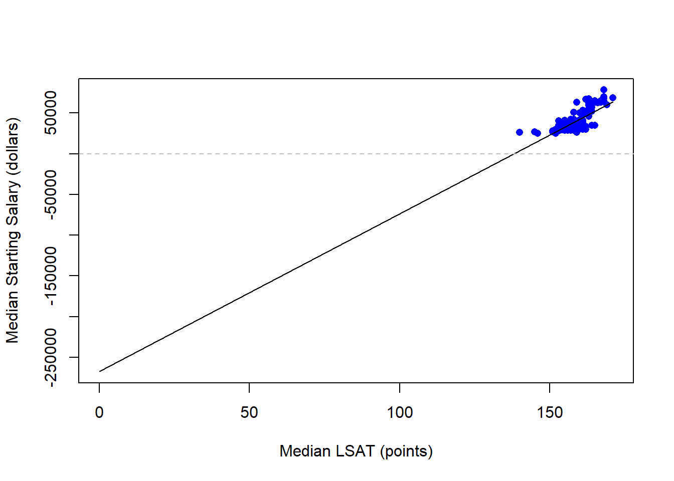
\[\hat\beta_0 = -267460.1\]
The expected value of Y when X = 0
\[\widehat{SALARY}_i = -267460.1 + 1936.66 \; (0)\]
As in previous examples, this intercept doesn’t make sense because none of the classes in our sample had a median LSAT score of zero.
Slope term
\[\hat\beta_1 = 1936.66\]
The expected change in Y in response to a one-unit change in X
\[\frac{\Delta\widehat{SALARY}_i}{\Delta LSAT} = \hat\beta_1 = 1936.66\]
We can therefore conclude that an additional point in median LSAT score will result in a 1936.66 dollar increase in median starting salary on average.
Other Regression Diagnostics
Every part of the dependent variable that the deterministic component of our model cannot explain ends up in the residual (i.e., garbage can)
\[salary_i = \hat\beta_0 + \hat\beta_1 \; LSAT_i + e_i\]
\[e_i = salary_i - \hat\beta_0 - \hat\beta_1 \; LSAT_i\] \[e_i = salary_i - -267460.1 - 1936.66 \; LSAT_i\]
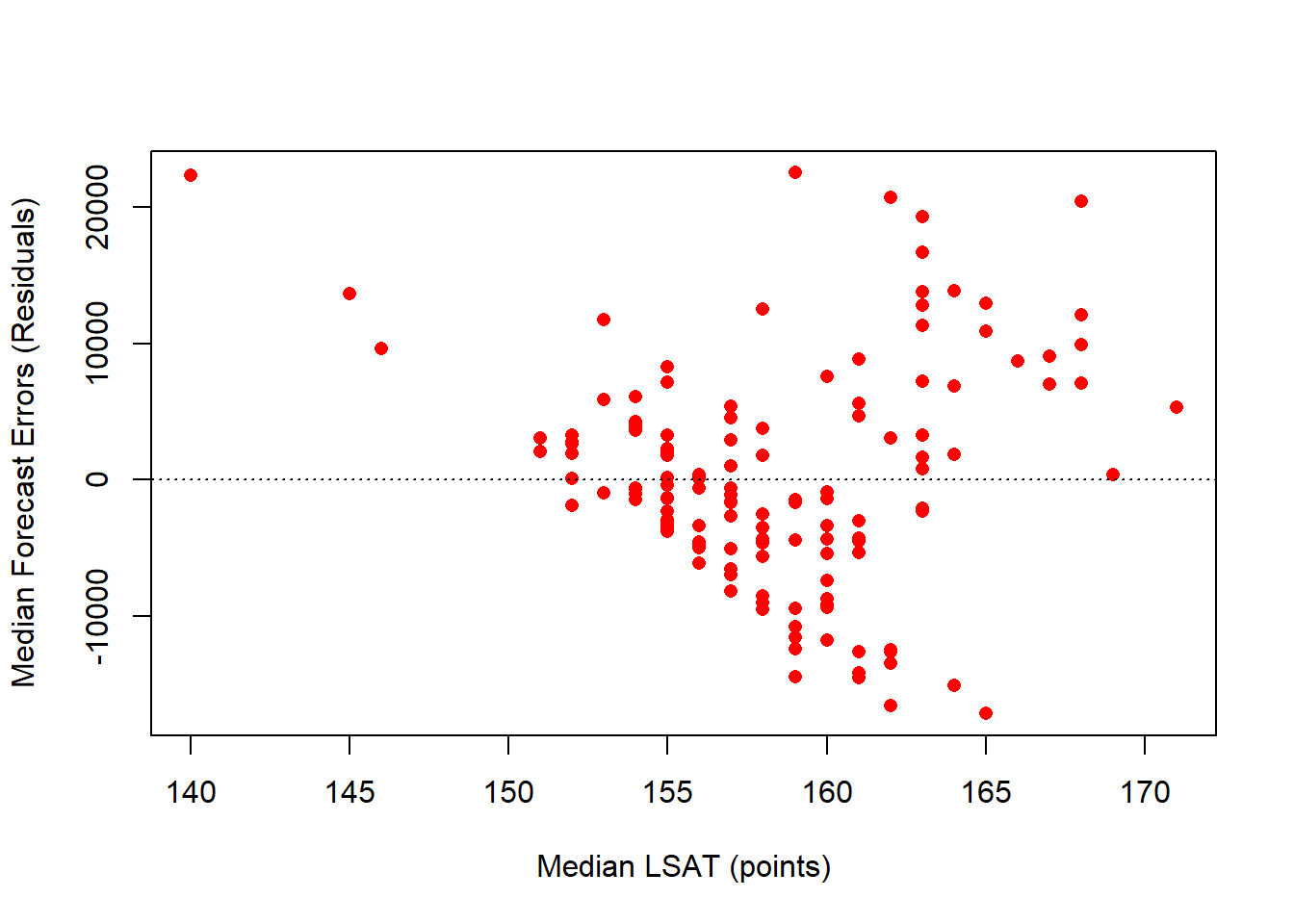
These residuals are essentially our forecast errors. The standard error of our forecast errors (the contents of our Garbage Can) is given by:
\[S_{YX} = \sqrt{ \frac{\sum e^2_i}{n-2}}\]
## [1] 8199.488The Infamous \(R^2\) is nothing more than the percentage of the variation in the dependent variable explained by the model.
\[R^2 = \frac{ESS}{TSS}\]
no more, no less…
## [1] 0.5550378