7.1 A Simple Linear Regression Model
A Linear Regression model is a line equation.
The simplest example of a line equation is:
\[Y_i=\beta_0+\beta_1X_i\]
The betas, \(\beta_0\) and \(\beta_1\) are called line coefficients.
\(\beta_0\) is the constant or intercept term
\(\beta_1\) is the slope term - it determines the change in Y given a change in X
\[\beta_1=\frac{Rise}{Run}=\frac{\Delta Y_i}{\Delta X_i}\]
7.1.1 What does a regression model imply?
\[Y_i=\beta_0+\beta_1X_i\]
When we write down a model like this, we are imposing a huge amount of assumptions on how we believe the world works.
First, there is the Direction of causality. A regression implicitly assumes that changes in the independent variable (X) causes changes in the dependent variable (Y). This is the ONLY direction of causality we can handle, otherwise our analysis would be confounded (what causes what) and not useful.
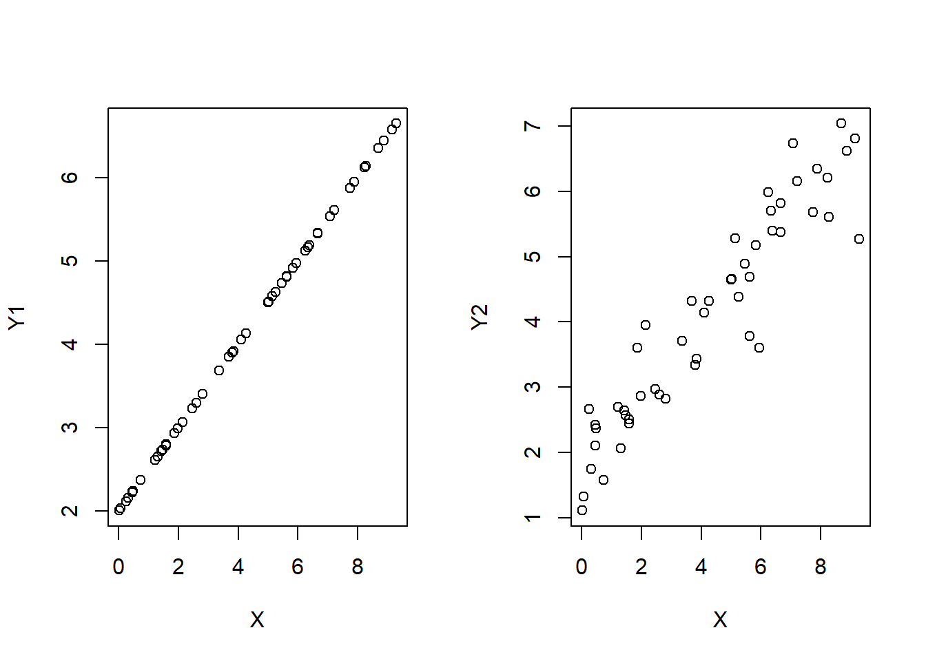
Second, The equation assumes that information on the independent variable (X) is all the information you need to explain the dependent variable (Y). In other words, if we were to look at pairs of observations of X and Y on a plot, then the above equation assumes that all observations (data points) line up exactly on the regression line.
This would be great if the observations look like the figure on the left, but not if they look like the figure on the right.

It would be extremely rare for the linear model (as detailed above) to account for all there is to know about the dependent variable Y…
There might be other independent variables that explain different parts of the dependent variable (i.e., multiple dimensions). (more on this next chapter)
There might be measurement error in the recording of the variables.
There might be an incorrect functional form - meaning that the relationship between the dependent and independent variable might be more sophisticated than a straight line. (more on this next chapter)
There might be purely random and therefore totally unpredictable variation in the dependent variable.
This last item can be easily dealt with!
Adding a stochastic error term (\(\varepsilon_i\)) to the model will effectively take care of all sources of variation in the dependent variable (Y) that is not explicitly captured by information contained in the independent variable (X).
7.1.2 The REAL Simple Linear Regression Model
\[Y_i=\beta_0+\beta_1X_i+\varepsilon_i\]
The Linear Regression Model now explicitly states that the explanation of the dependent variable \((Y_i)\) can be broken down into two components:
A Deterministic Component: \(\beta_0+\beta_1X_i\)
A Random / Stochastic / Explainable Component: \(\varepsilon_i\)
Lets address these two components in turn.
The Deterministic Component
\[\hat{Y}_i=\beta_0+\beta_1X_i\]
The deterministic component delivers the expected (or average) value of the dependent variable (Y) given a values for the coefficients (\(\beta_0\) and \(\beta_1\)) and a value of the dependent variable (X).
Since X is given, it is considered deterministic (i.e., non-stochastic)
In other words, the deterministic component determines the mean value of Y associated with a particular value of X. This should make sense, because the average value of Y is the best guess.
Technically speaking, the deterministic component delivers the expected value of Y conditional on a value of X (i.e., a conditional expectation).
\[\hat{Y}_i=\beta_0+\beta_1X_i=E[Y_i|X_i]\]
The Unexpected (Garbage Can) Component
\[\varepsilon_i=Y_i-\hat{Y}_i\]
Once we obtain the coefficients, we can compare the observed values of \(Y_i\) with the expected value of \(Y_i\) conditional on the values of \(X_i\).
The difference between the true value \((Y_i)\) and the expected value \((\hat{Y}_i)\) is by definition… unexpected!
This unexpected discrepancy is your prediction error - and everything your deterministic component cannot explain is deemed random and unexplainable.
If a portion of the dependent variable is considered random and unexplainable - then it gets thrown away into the garbage can (\(\varepsilon_i\)).
This is a subtle but crucial part of regression modeling…
Your choice of the independent variable(s) dictate what you believe to be important in explaining the dependent variable.
The unimportant (or random) changes in the dependent variable that your independent variables cannot explain end up in the garbage can by design.
Therefore, the researcher essentially chooses what is important, and what gets thrown away into the garbage can.
YOU are the researcher, so YOU determine what goes into the garbage can!