4.3 Application 2: A Sampling Distribution with an Unknown Population
In most applications, we will not be as lucky as in the first application and we will know nothing about the underlying population. We won’t know the distributional properties of the population, we won’t know any of the population parameters… nothing. The beauty of the CLT is that this doesn’t matter. We can still apply the CLT to set the stage for statistical inference.
In light of school closings back in 2020, the city of Philadelphia considered sending out $100 EBT cards to every student registered in public school.
A key question at the beginning of deliberation is how much would this policy cost?
There are 352,272 families in Philadelphia, and the city has records on how many students are registered in public schools.
- Suppose it is too costly (at the initial stage) to determine the total number of children.
If we knew the average number of children registered per family, we can get an estimate of the cost of the policy.
Suppose we are omniscient…
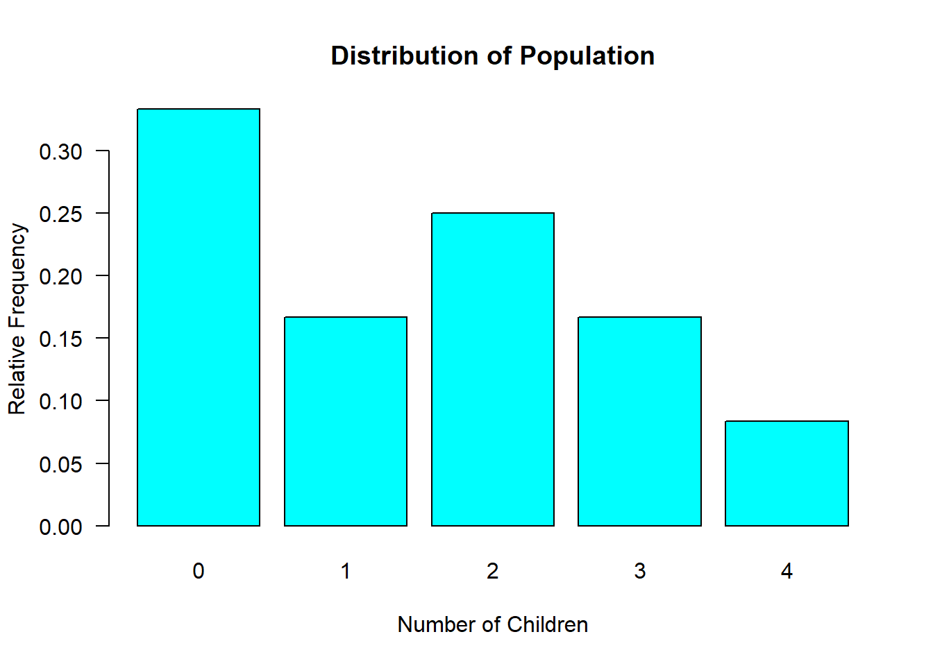
- The POPULATION average number of children per family is… \[\mu = 1.5\] \[\sigma = 1.38\]
NOTE: We do not know these population parameters. I am simply stating them here so we can refer to them later for verification. In reality, we will never know these population parameters. That’s why we need inferential statistics.

4.3.1 The Sample
Since it is too costly to examine the entire population (at the initial stage), we draw a single sample.
We use the sample to calculate sample statistics
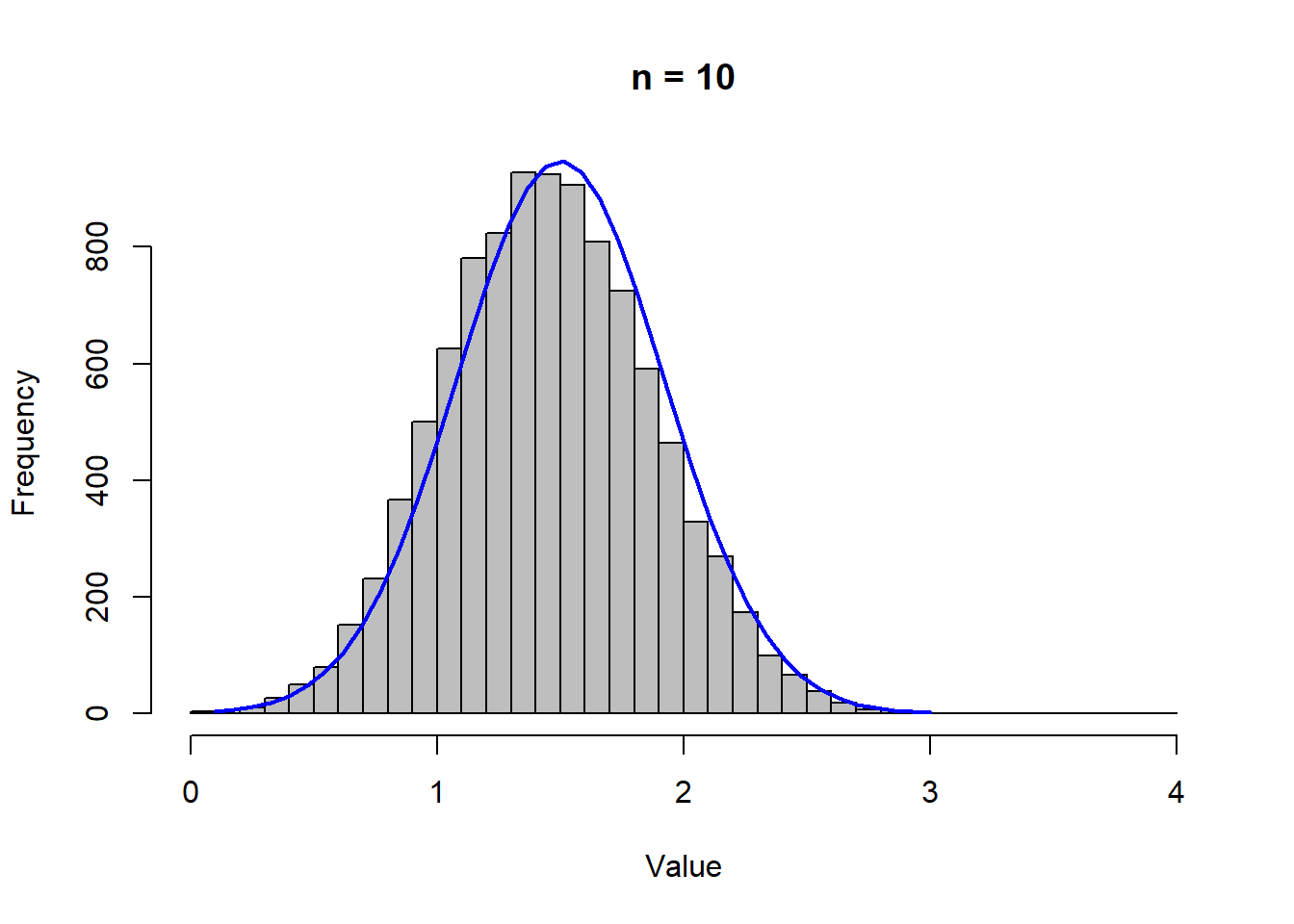
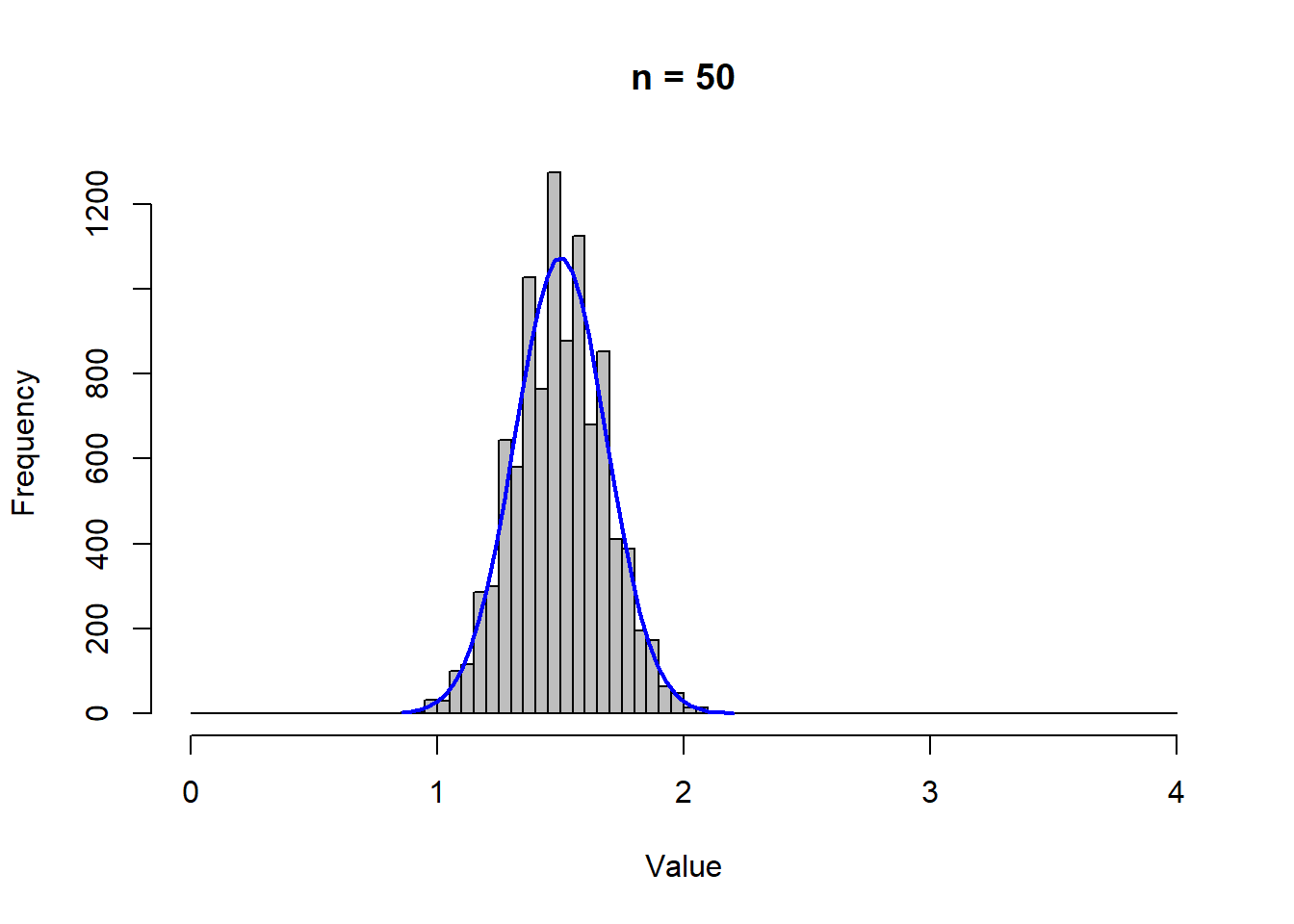
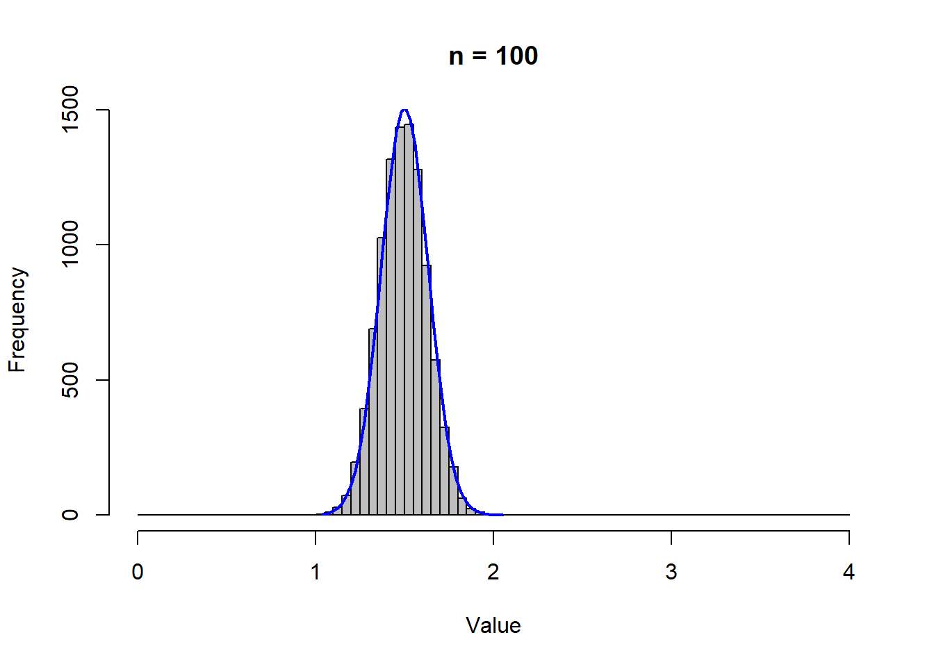
Since the sample is randomly drawn from the population, the sample statistics are randomly drawn from a sampling distribution.
The characteristics of the sampling distribution depends on the sample size \(n\).


The figures above show sampling distributions of various sample sizes. Note that all of these distributions are centered around the same number (of 1.5), and the dispersion around the mean is getting smaller as \(n\) is getting larger. In other words, the standard deviation \(\sigma / \sqrt{n}\) is getting smaller because \(n\) is getting larger (while \(\sigma\) remains unchanged).