4.2 Application 1: A Sampling Distribution with a Known Population
The first application presents sampling distributions for a random process where we know the underlying process of the population: The rolling of two die.
Suppose you worked for a gaming commission and placed in charge of making sure the dice at a casino were fair. We know that the (population) average roll of 2 fair die is 7 while the standard deviation is 2.45.4
It wouldn’t be fair for you to test a set of dice by rolling them once because there is a large probability of rolling a number other than 7. In particular, there are 36 possible outcomes of rolling two die and only 6 of those outcomes equal 7. This means that although 7 is the highest probability single outcome, there is a much higher probability of rolling a number other than 7 (ever play craps?).

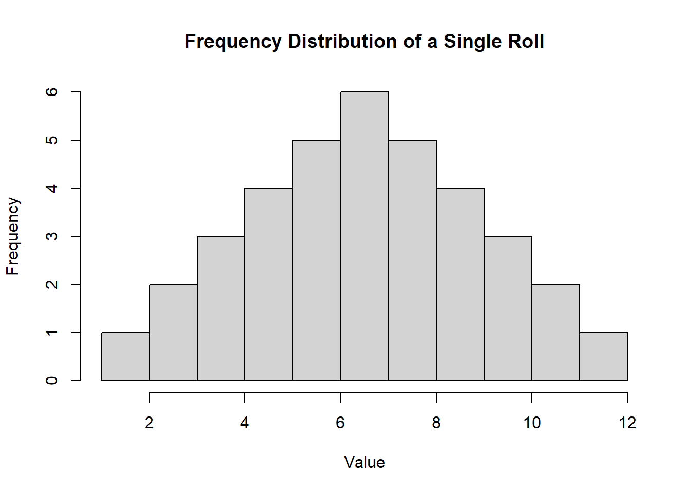
The figure above is the population distribution of rolling two die. The average (mean) value is 7, the range of possible outcomes are between 2 and 12, and the standard deviation is a number that represents the dispersion of individual values around the mean. If you were to roll two die, then the outcome of that roll is conceptually a draw from this distribution.
Since we don’t want to wrongfully accuse the casino of cheating, we need to roll the dice a few times to get an idea of what the average roll value is. If it is fair dice, then we know they will roll a 7 on average - but that means we would need to roll the dice an infinite amount of times to achieve this. To be realistic, lets settle on a number of rolls to be generally given by \(n\). If we choose \(n=5\), then that means we roll the dice 5 times, record the roll each time, and then record the average. This is a sample average of a sample of size 5. We could do this for \(n=10\), \(n=30\), \(n=300\), etc.

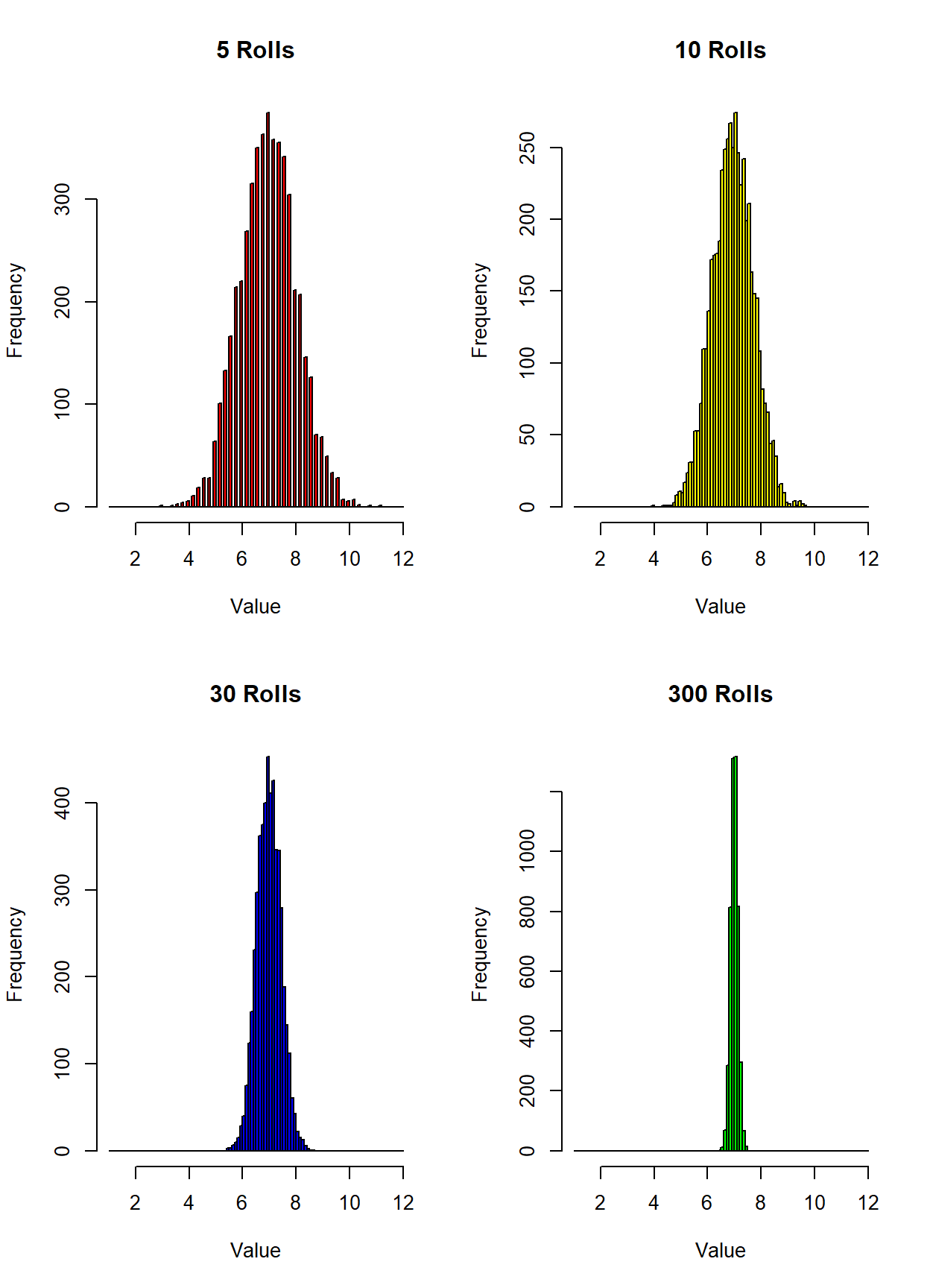
Figure 4.1: Sampling Distributions
The figure is illustrating four potential sampling distributions. For example, if you were to collect a sample of 5 rolls, then you would technically be drawing a sample average from the distribution in the upper left. On the other hand, if you decide to roll the dice 300 times, then you are technically drawing a sample average from the distribution in the lower-right.
There are two main takeaways from the above illustration.
Sampling distributions appear to approximate normal distributions. The normal distribution is the classic bell-curve distribution that tends to mysteriously show up in empirical analyses. The CLT is the reason why. Note that even though the original distribution didn’t look like a normal distribution at all, you still can construct sampling distributions that appear normal. This holds regardless of the initial population distribution (check out the video about rabbits and dragons on the course website if you don’t believe me).
Sampling distributions become more normal and have a lower standard deviation when the sample size gets bigger. Notice that as the sample size goes up, the distributions become narrower. This means that when there is a big sample size there is a very low probability that your going to see sample averages near 2 or 12. This should make sense: If you roll two dice 300 times and take the average, there is no way you are going to record a sample average of 2 unless you roll snake eyes 300 times in a row. As the sample size increases, the extreme events start getting diluted. This reduces the standard deviation of the sampling distribution.
The sampling distributions (for \(n \geq 30\)) are distributed normal with mean \(\mu\) and standard deviation \(\sigma / \sqrt{n}\). Technically this means that your random sample will produce a random outcome (a sample mean) which we denote \(\bar{X}\).
\[ \bar{X} \sim N \left( \mu, \frac{\sigma}{\sqrt{n}} \right) \]
You can see these two properties in the four sampling distributions illustrated above. All four sampling distributions are centered around 7, which is the population mean. As sample size gets larger, the sampling distributions get narrower around the population mean. This illustrates why a larger sample has a better shot at becoming a better representation of the population.
The mean of a single dice throw is 3.5, \[ 3.5 = (1 + 2 + 3 + 4 + 5 + 6) / 6\] and the expected value of two independent dice is the sum of expected values of each die. Standard deviation can be calculated using this mean value and the formula presented earlier.↩︎