6.3 Two-sided vs One-sided Test

\[H_0:\mu=4.5 \quad versus \quad H_1:\mu\neq 4.5\]

The hypothesis test considered above is known as a two-sided test because the null gets rejected if the mean of the sample is either significantly greater than or less than the value stated in the null hypothesis. If you notice from the illustrations above, a two-sided test has TWO rejection regions - one in each tail (hence the name). Note that this is also why we calculated critical values using half of the value of \(\alpha\) and doubled the calculated probability value in order to arrive at a p-value.

In the fast food example above, suppose we want to show that the service time increased. In other words, we want statistical evidence that the wait time actually increased from a previous time of 4.5 minutes. We can provide statistical evidence by rejecting a null hypothesis that the new population average wait time is 4.5 minutes or less. This scenario delivers us a one-sided hypothesis test.

\[H_0:\mu \leq 4.5 \quad versus \quad H_1:\mu> 4.5\]

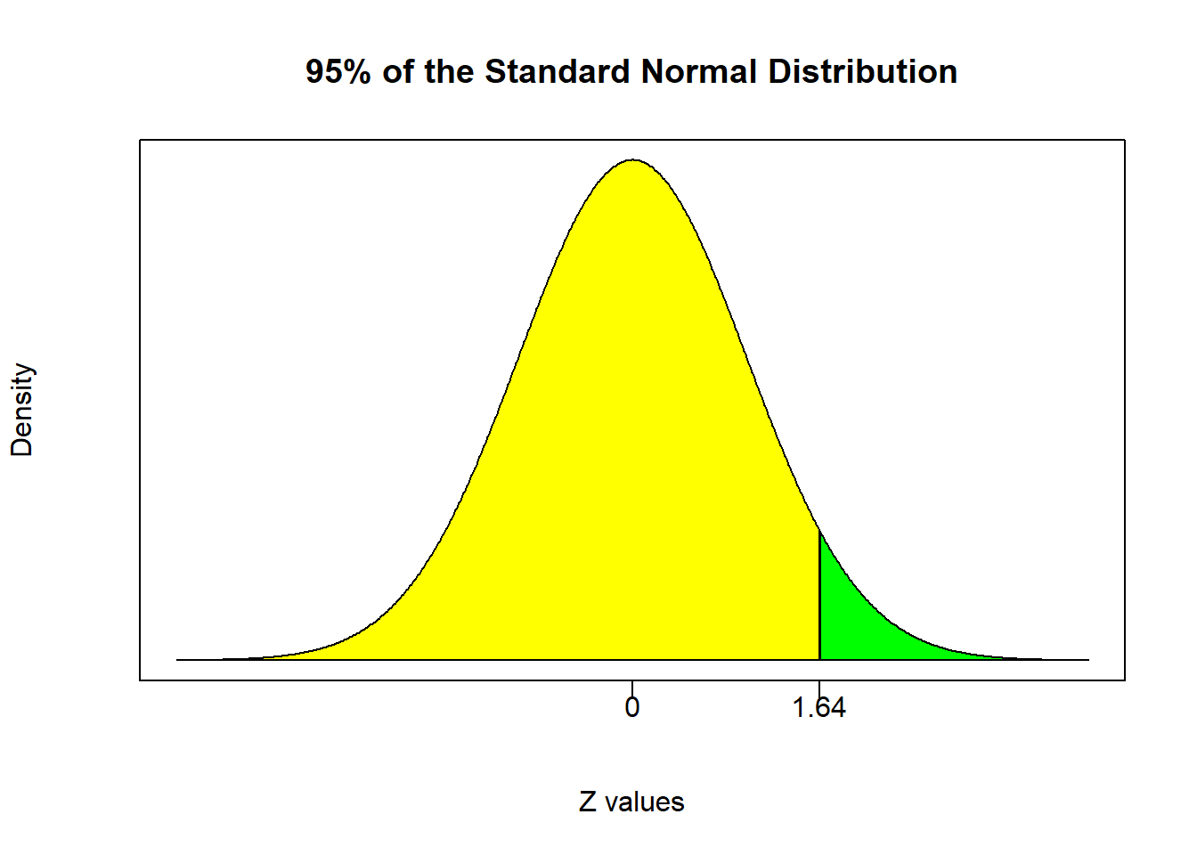
As the name implies, a one-sided hypothesis test only has one rejection region. This means that the entire value of \(\alpha\) is grouped into either the right or left tail. The tail containing the rejection region depends upon the exact specification of the hypothesis test.

The hypothesis test above is called a right-tailed test because the rejection region is in the right tail. To see this, consider several hypothetical sample averages and see if they are consistent with the null \(\mu \leq 4.5\).

• Suppose you observe \(\bar{X}=4\). Is this sample average consistent with \(\mu \leq 4.5\)?

• What about \(\bar{X}=2\)?

• What about \(\bar{X}=1\)?

Your answer should be yes to all of these sample averages. In fact, any sample average less than or equal to 4.5 is consistent with \(\mu \leq 4.5\).

Next, recall the test statistic under the null:

\[ Z = \frac{\bar{X}-4.5}{\left(\sigma / \sqrt{n} \right)}\]

For any of the hypothetical values considered above (4, 2, or 1), the test statistic would be a negative number. Since we said that all of these sample averages are consistent with the null being true, then we would never reject the null in any of these instances. Therefore, the rejection region cannot be in the left tail because that is where the negative values of the distribution reside. The rejection region must therefore be in the right tail. Only when a sample average is sufficiently greater than 4.5 is when we can consider rejecting the null.

Now that we already have the null and alternative hypotheses down as well as the test statistic under the null, the next step is to determine the critical value that divides the distribution into rejection and nonrejection regions.

# Fast Food Example Revisited
mu = 4.5
Xbar = 5.1
Sig = 1.2
n = 25

(Zstat = (Xbar - mu)/(Sig/sqrt(n)))

## [1] 2.5

# 95% confidence:
alpha = 0.05
(Zcrit = qnorm(alpha,lower.tail=FALSE))

## [1] 1.644854

# P-value:
(Pval = pnorm(Zstat,lower.tail=FALSE))

## [1] 0.006209665

# highest Confidence Level for rejection:
((1-Pval)*100)

## [1] 99.37903

If we conducted this hypothesis test at the 95% confidence level ($), you will see that the rejection region is the 5% of the curve in the right tail. That means you reject all test statistics greater than or equal to 1.64. Since our test statistic is 2.5, we can reject with 95% confidence. We can also conduct this hypothesis test using the p-value approach which delivers a p-value of 0.0062. This means that if we reject the null, we only incur a 0.62% chance of being wrong. This equivalently means that we can reject the null with up to 99.38% confidence.