8.1 Application: Explaining house price in a multiple regression
Let us revisit the relationship between house price and house size, but extend the regression model to include the number of bedrooms as a second independent variable.
Our PRF becomes:
\[Price_i=\beta_0+\beta_1Size_i+\beta_2Rooms_i+\varepsilon_i\]
Our SRF becomes:
\[Price_i=\hat{\beta}_0+\hat{\beta}_1Size_i+\hat{\beta}_2Rooms_i+e_i\]
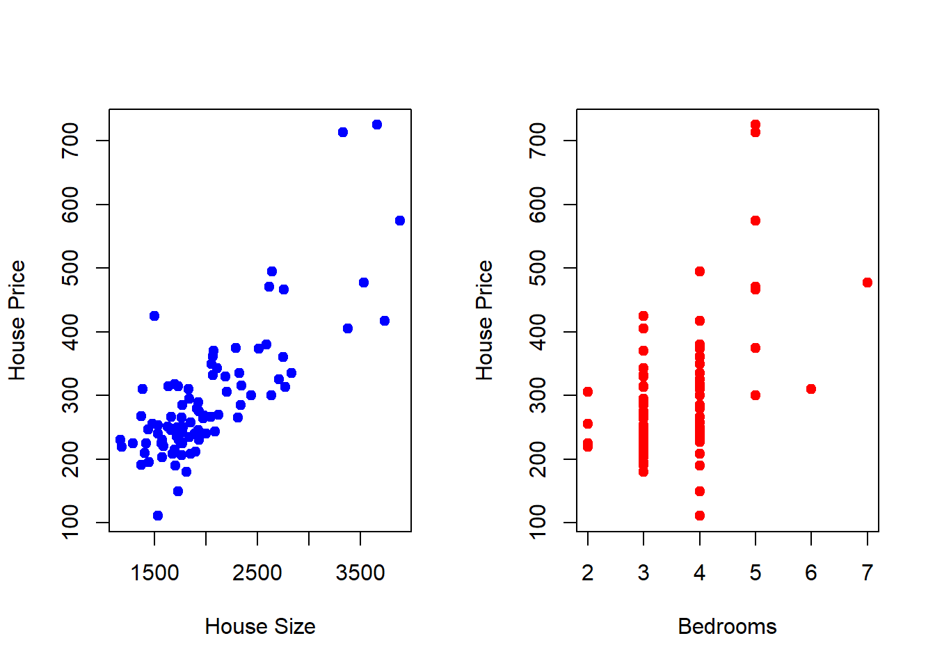
To visualize what we are about to do, lets start with scatter plots looking at the relationships between the dependent variable and each independent variable.
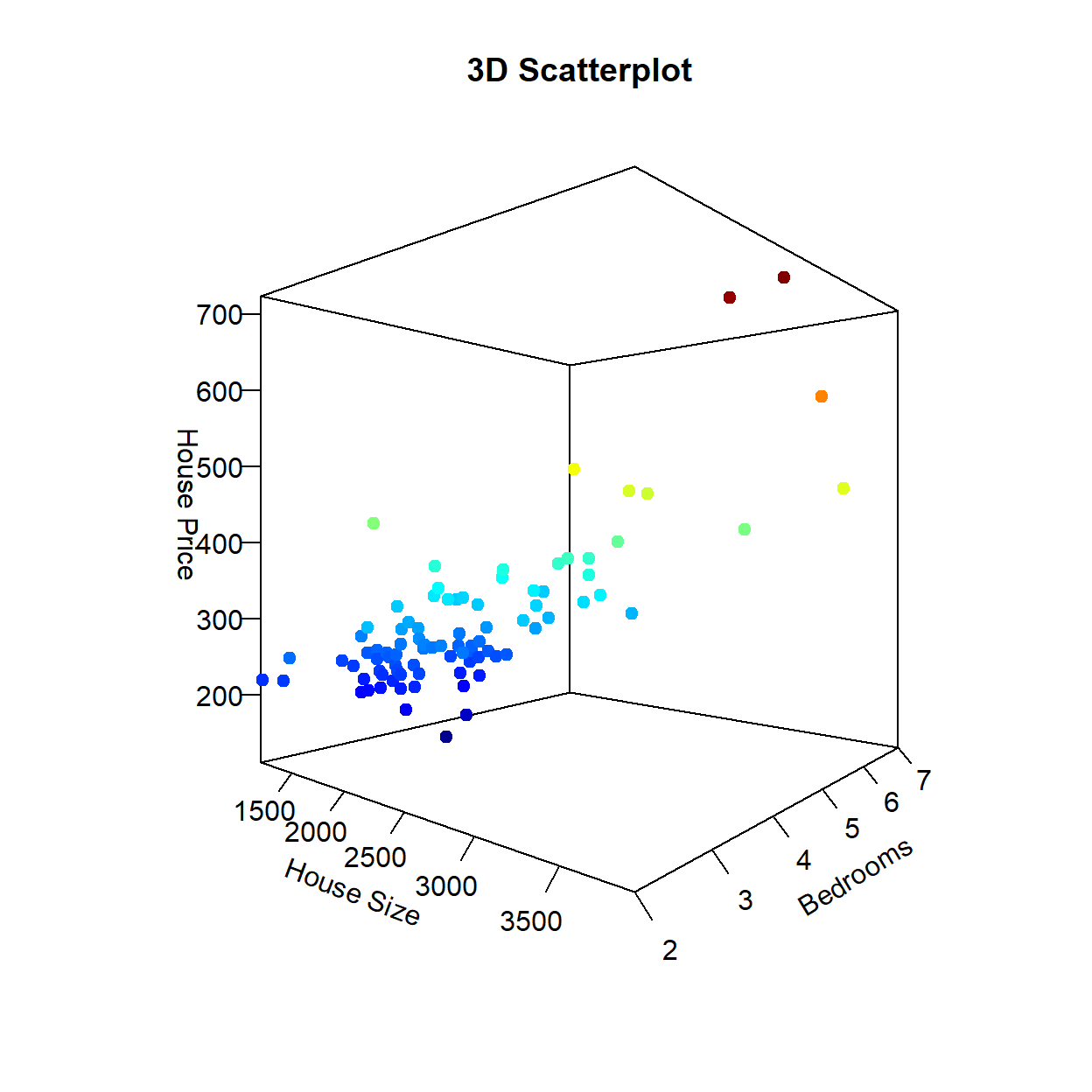
The figure on the left is the scatter plot between the House Price and House Size. This positive relationship is exactly what we have looked at previously. The figure on the right is the scatter plot between the same House Price but the number of bedrooms each house has. This figure illustrates that the houses in our sample have between 2 and 7 bedrooms (with no half-rooms), and homes with more bedrooms generally have higher prices (as expected). Note that we are looking at the same dependent variable along different dimensions. We can combine these dimensions into a singe (3-Dimensional) figure to see how the relationships between the dependent variable and each independent variable appear simultaneously.
data(hprice1,package='wooldridge')
Y <- hprice1$price
X1 <- hprice1$sqrft
X2 <- hprice1$bdrms

par(mfrow = c(1,2))
plot(X1,Y, col = "blue",
          pch = 19, cex = 1,
          xlab = "House Size", ylab = "House Price")
plot(X2,Y, col = "red",
          pch = 19, cex = 1,
          xlab = "Bedrooms", ylab = "House Price")
scatter3D(X1, X2, Y, pch = 19, cex = 1, phi = 0,
          colkey=FALSE, ticktype = "detailed",
          xlab = "House Size", ylab = "Bedrooms",
          zlab = "House Price", main = "3D Scatterplot")
For comparison, suppose that we consider these independent variables one at a time in a simple regression. In particular, we can examine one simple regression model where House Size is the only independent variable, and another simple regression model where Bedrooms is the only independent variable.
REG1 <- lm(hprice1$price ~ hprice1$sqrft)
coef(REG1)
## (Intercept) hprice1$sqrft
## 11.204145 0.140211REG2 <- lm(hprice1$price ~ hprice1$bdrms)
coef(REG2)## (Intercept) hprice1$bdrms
## 72.23111 62.02456The regression that only considers house size has a slope coefficient of 0.14. Remember that since house price was denoted in thousands of dollars and house size was denoted in square feet, this slope coefficient states that an additional square foot of house size will increase the average house price by $140.
The regression that only considers number of bedrooms has a slope coefficient of 62. This slope coefficient states that an additional bedroom will increase the average house price by $62,000.
While the results from these two simple regressions make sense, we need to realize that a simple regression model only considers a single independent variable to be important (and throws all of the other information into the garbage can). This means that the first regression takes no notice of the number of rooms a house has, while the second regression takes no notice of the size of the home. Since it is reasonable to assume that bigger homes have more bedrooms, then a regression model that is only given one of these pieces of information might be overstating the quantitative impact of the single independent variable.
To illustrate this, let us run a multiple regression model where both house size and number of bedrooms are considered.
REG3 <- lm(price ~ sqrft + bdrms, data = hprice1)
coef(REG3)
## (Intercept) sqrft bdrms
## -19.3149958 0.1284362 15.1981910The slope with respect to house size is now 0.128 (down from 0.14) while the slope with respect to number of bedrooms is now 15.2 (down from 62). In order to make sense of these changes, let us explicitly interpret these slope coefficients within the context of a multiple regression model (where we can hold all other independent variables constant).
Holding number of bedrooms constant, an additional square foot of house size will increase a house price by $128, on average.
Holding house size constant, an additional bedroom will increase a house price by $15,200, on average.
The power of a multiple regression comes through when you look at the second slope interpretation. Multiple regression allows us to consider two houses that have the same house size but one house has an additional bedroom. In other words, imagine building a wall that turns one bedroom into two smaller bedrooms. This will increase the expected house price by $15,200, but this is much smaller than the simple regression relationship of $62,000. This is because the simple regression could not differentiate the impact of a bedroom from the impact of an increase in house size. The multiple regression model can.
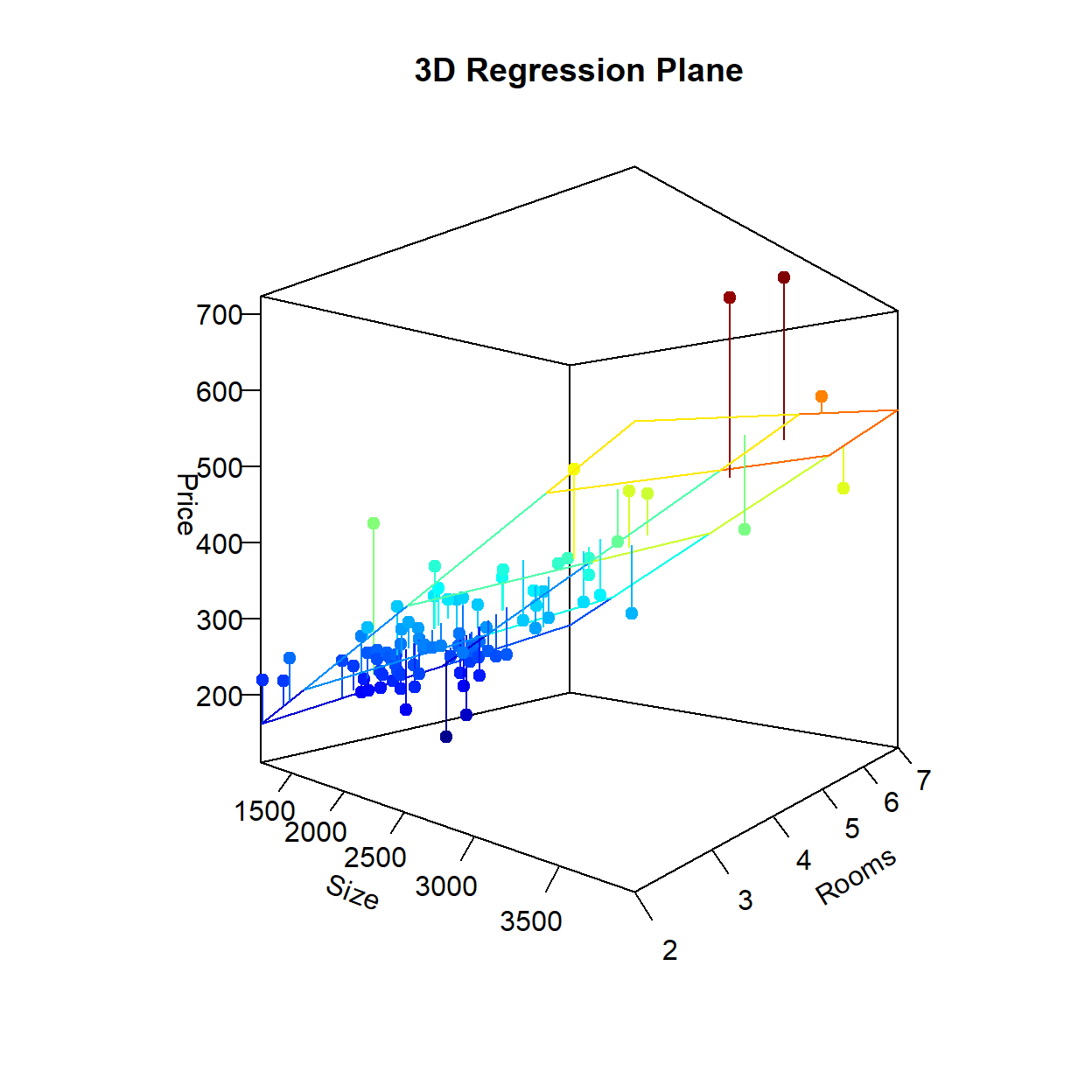
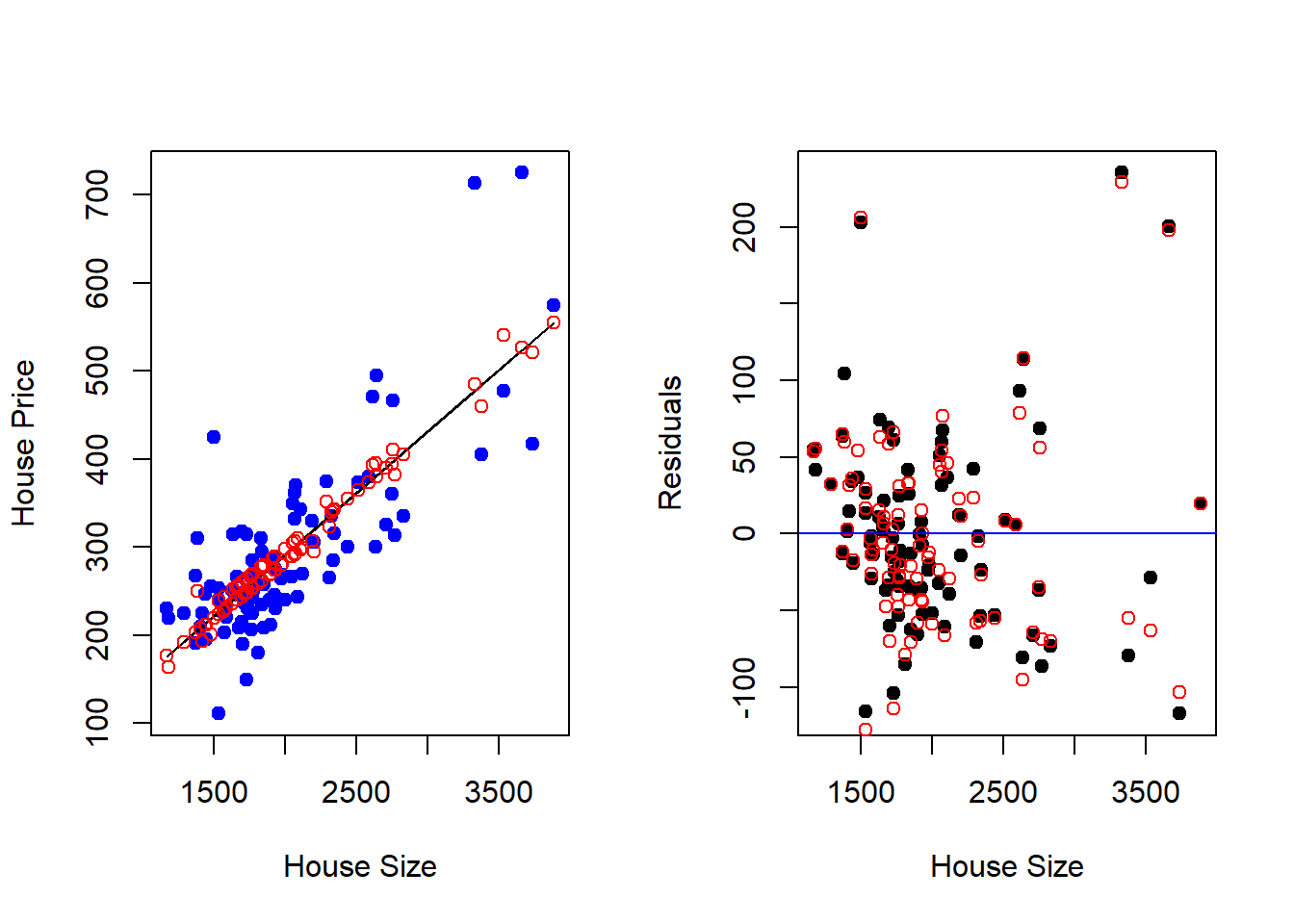
The final figure shows the 3-dimensional regression line (i.e., plane) that best fits the sample. You can see that considering multiple dimensions increases the performance of the deterministic component of the model and therefore reduces the amount of information that goes into the garbage can as unpredictable. This can be shown in the last picture that only looks at the relationship from the “Size” dimension. In the figure on the left, the blue dots are the observations in the data, the black line is the regression line from the simple regression model (without Bedrooms), while the red dots are the model predictions from the multiple regression model with Bedrooms included as an additional independent variable. Notice how this allows the regression predictions to veer off of a straight line. This results in slightly less prediction errors showing up in your garbage can - as illustrated in the figure on the right.

par(mfrow = c(1,2))
plot(hprice1$sqrft,hprice1$price, col = "blue",
          pch = 19, cex = 1,
          xlab = "House Size", ylab = "House Price")
lines(hprice1$sqrft,fitted(REG1))
points(hprice1$sqrft,fitted(REG3),col = "red")

plot(hprice1$sqrft,residuals(REG1), col = "black",
          pch = 19, cex = 1,
          xlab = "House Size", ylab = "Residuals")
points(hprice1$sqrft,residuals(REG3),col = "red")
abline(h = 0,col="blue")
8.1.1 The Importance of “Controls”
One very important item to point out in the last application is exactly why the coefficient on number of bedrooms dropped from $62,000 to $15,200 when the size of the house was added to the regression. The reason can be broken up into two categories.
2. “All Else Equal” in a Multiple Regression is more than just words
A multiple regression can separately identify the impact of each independent variable on the dependent variable.
Put together, these two items suggest that when two independent variables are correlated, then they should both appear in the regression model. If not, then the correlation between an included independent variable and an omitted independent variable might lead to omitted variable bias. This is what we saw above in the regression with only number of bedrooms as an independent variable. The coefficient of $62,000 is giving you the combined impact of an additional room and a bigger house. When you add house size as another independent variable, you are now able to determine the expected increase in house price for an additional bedroom holding house size constant.
Bottom line is that even though you are concerned with the results from a particular independent variable, it is important to try and include all independent variables that might be correlated with the independent variable of interest. This attempts to alleviate omitted variable bias.