5.5 Concluding Applications
5.5.1 Light Bulbs (Last Time)
Let’s go back one last time to our light bulb example
load("C:/Data/MBA8350/Lightbulb.Rdata")
(n = length(Lifetime))
## [1] 60(Xbar = mean(Lifetime))## [1] 907.5552(S = sd(Lifetime))## [1] 78.96741We have the following information from our sample:
\[\bar{X}=907.6, \quad n = 60, \quad S = 78.967\]
Use the above information to calculate a 95% confidence interval around the population average lifespan of the light bulbs you have left to sell. You can put this on information on the box!
alpha = 0.05
df = n-1
t = -qt(alpha/2,df)

(left = Xbar - t * S / sqrt(n))
## [1] 887.1557(right = Xbar + t * S / sqrt(n))## [1] 927.95465.5.2 Returning to the Philadelphia School Policy Application
Let us return to the Philadelphia school policy example to provide one final discussion of a confidence interval. This application may appear redundant, but it is intended to provide an alternative approach to the confidence interval concept. It has helped students in the past, so it might do some good.
In early February 2020, the city of Philadelphia considered sending out $100 EBT cards to every student registered in public school due to the school closings brought on by the pandemic.
How much would this policy cost?
The Frame
There are 352,272 families in Philadelphia, and the city has records on how many students are registered in public schools.
However, suppose it is too costly (at this stage) to determine the total number of children registered in public schools. If we knew the average number of children registered per family, we can get an estimate of the cost of the policy.
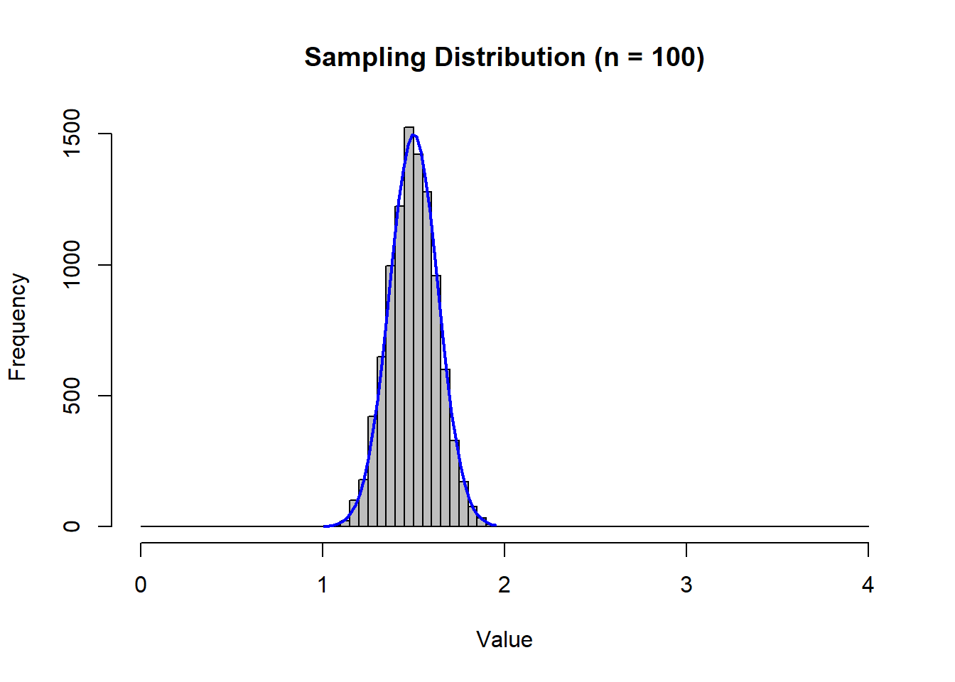
Since it is too costly to examine the entire population (at the moment), we draw a single sample and use the sample to calculate sample statistics. Since the sample is randomly drawn from the population, the sample statistics are randomly drawn from a sampling distribution.
Your Sample
Once you determine a sample size \((n)\), you get one random draw from the appropriate sampling distribution.
The distribution is approximately normal
The mean is \(\mu\)
The standard deviation \(\sigma/\sqrt{n}\)
We use this information and our sample characteristics to say something about the population parameters…
Suppose you select a sample of \(n=100\) families and calculate
\[Xbar = 1.7\]
\[S = 1.5\]
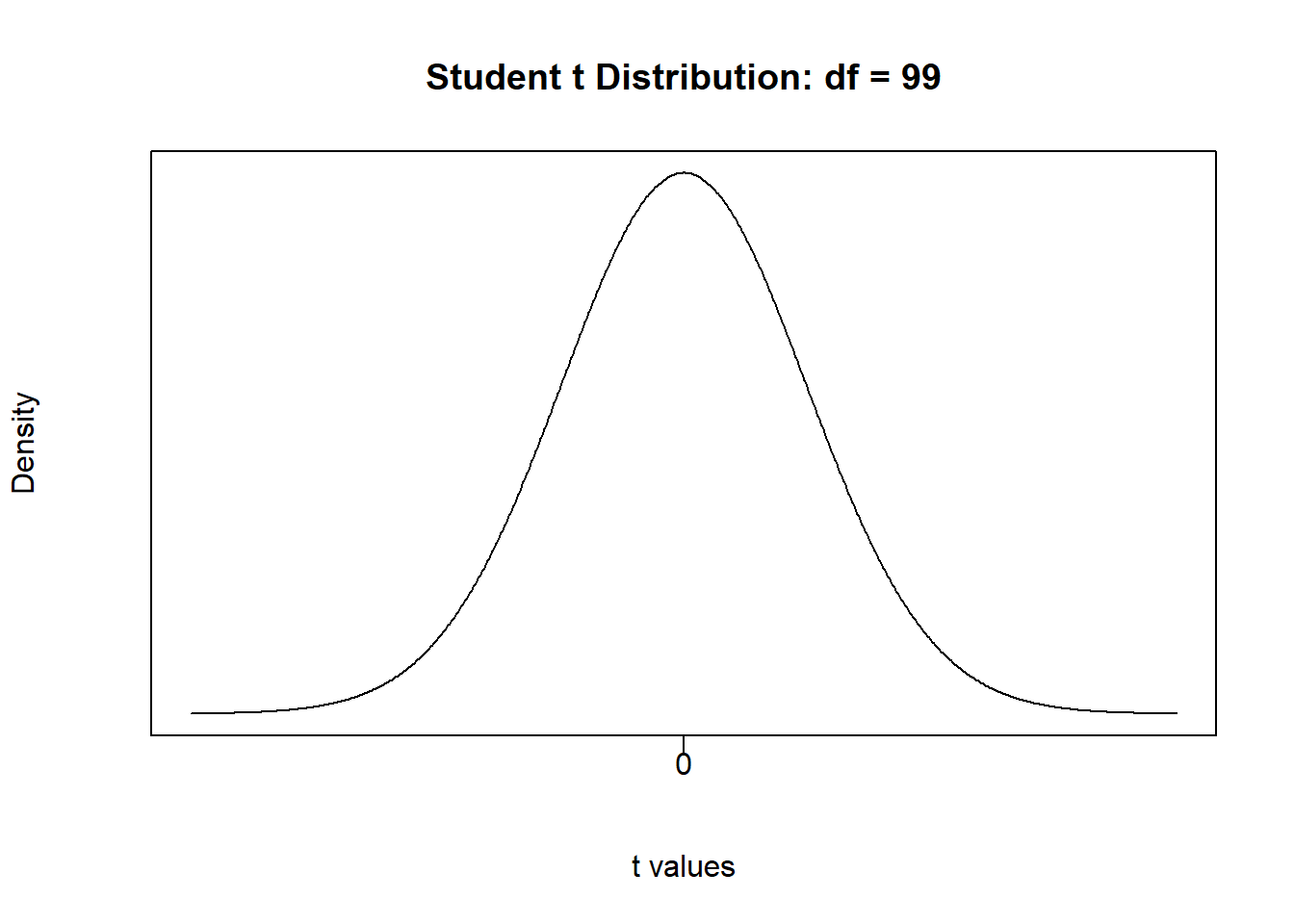
Since we have an estimate of the population standard deviation from our sample, our sampling distribution is now a t distribution with \(n-1 = 99\) degrees of freedom.
\[ t = \frac{\bar{X}-\mu}{S/\sqrt{n}}=\frac{1.7-\mu}{1.5/\sqrt{100}}\]
What we know…
CLT: the true population average is the central point of our sampling distribution
We can choose an arbitrary level of confidence \((1-\alpha)\) to limit where we think our statistic from a single draw will fall.
\[Pr(-t^* \leq \frac{1.7-\mu}{1.5/\sqrt{100}} \leq t^*) = 1-\alpha\]
Suppose we want 95% confidence \((\alpha = 0.05)\)
(tcrit <- qt(0.05/2,99))## [1] -1.984217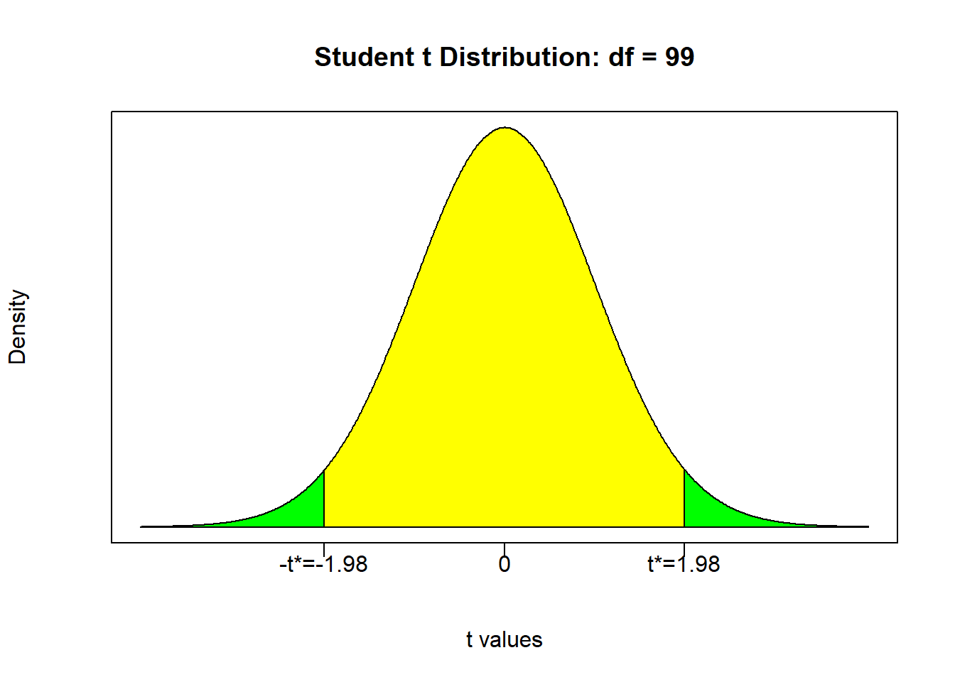
What we DON’T know…
We don’t know the numerical value of \(\mu\)…
We don’t know where our value of \(\bar{X}\) falls in relation to \(\mu\)
\(\bar{X}=\mu\)?
\(\bar{X}>\mu\)?
\(\bar{X}<\mu\)?
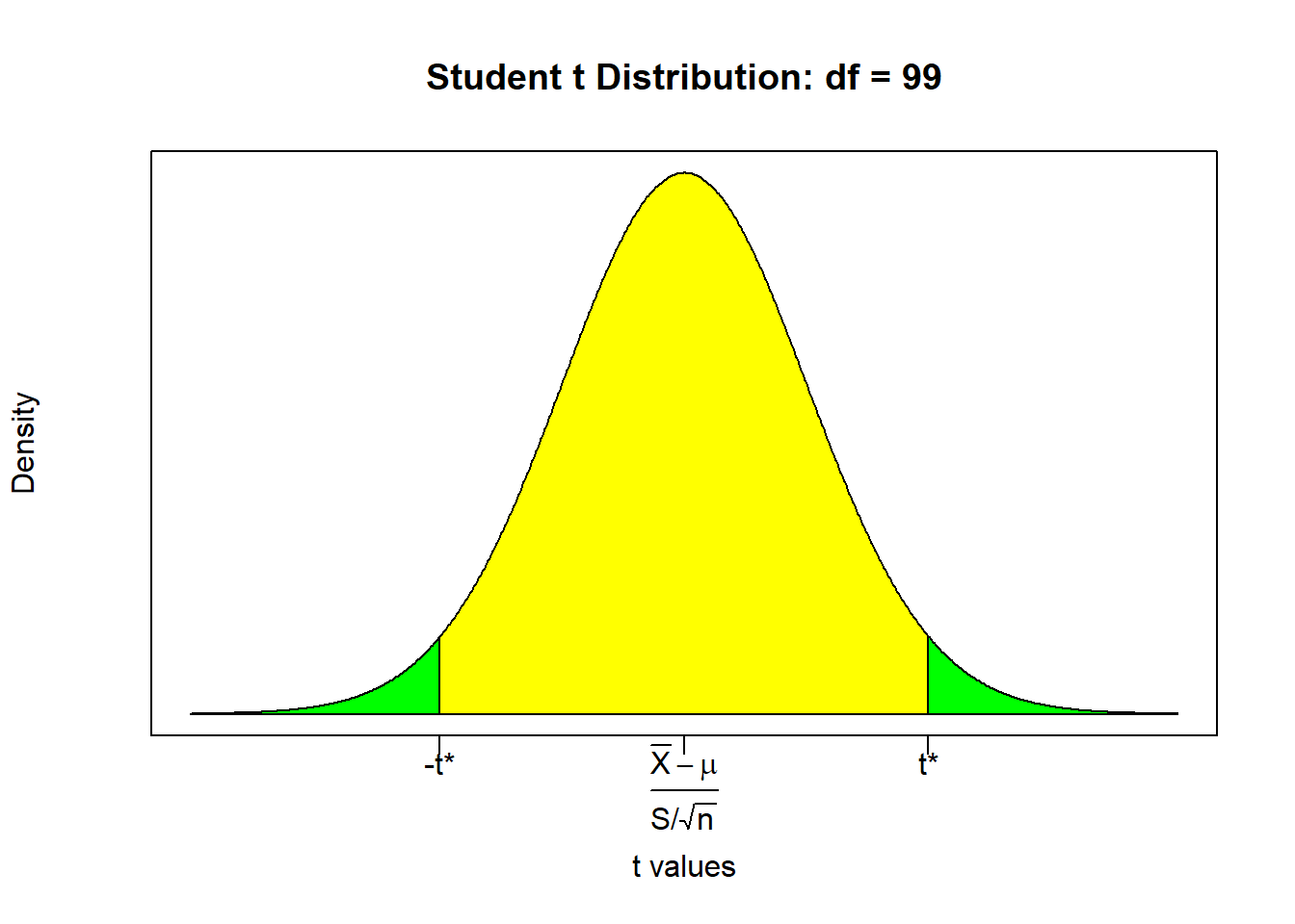
The fact that we don’t know where \(\bar{X}\) is in relation to \(\mu\) is why we end up with an interval around where we think the population parameter resides.
\[Pr(\bar{X}-t^* \frac{S}{\sqrt{n}} \leq \mu \leq \bar{X}+t^* \frac{S}{\sqrt{n}}) = 1-\alpha\]
\[Pr(1.7-1.98 \frac{1.5}{\sqrt{100}} \leq \mu \leq 1.7+1.98 \frac{1.5}{\sqrt{100}}) = 0.95\]
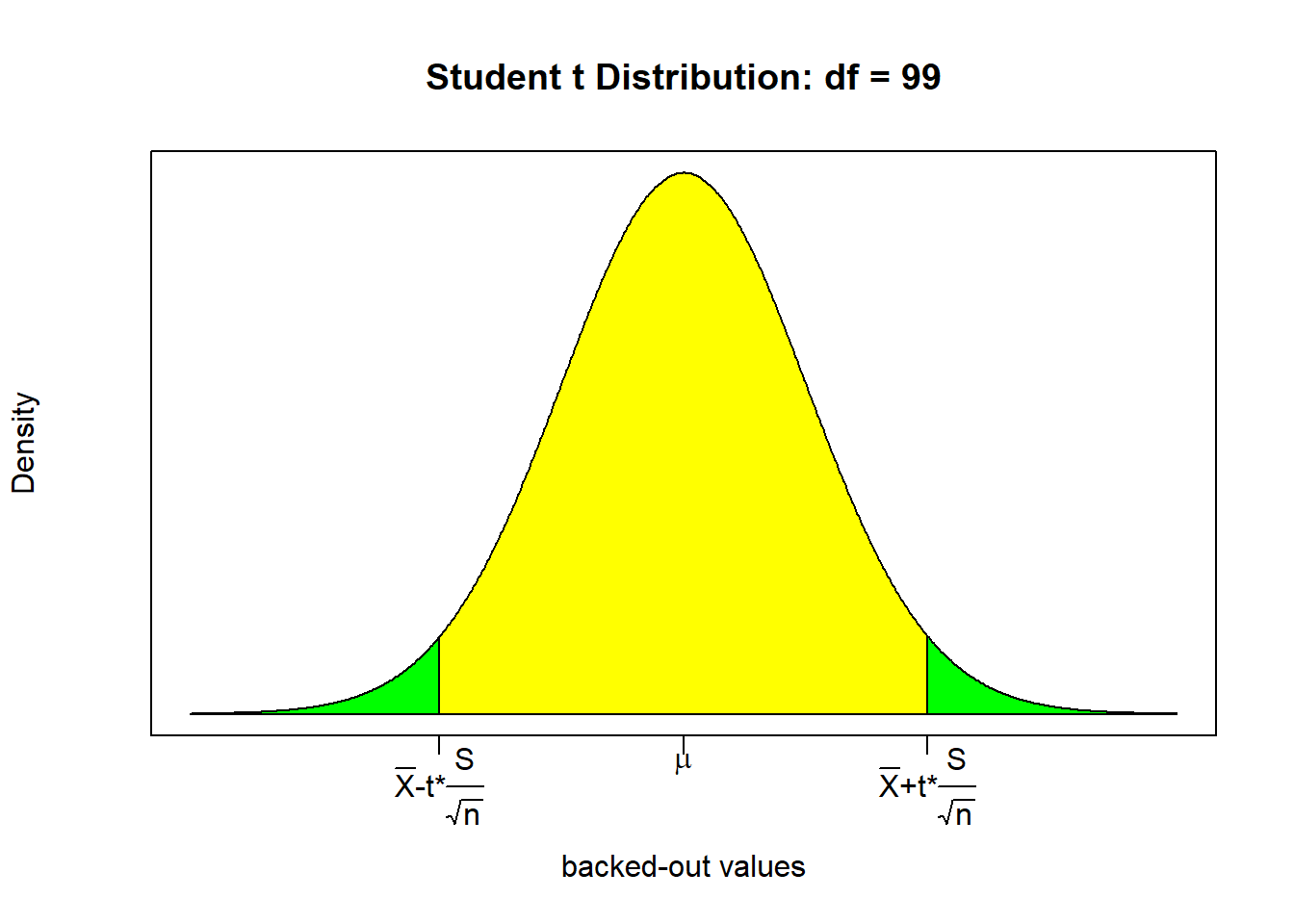
Xbar = 1.7; S = 1.5; n = 100; AL = 0.05
tcrit <- -qt(AL/2,n-1)

(LFT <- Xbar - tcrit * S / sqrt(n))
## [1] 1.402367(RHT <- Xbar + tcrit * S / sqrt(n))## [1] 1.997633\[Pr(1.40 \leq \mu \leq 2.00) = 0.95\]
With 95% confidence, the average number of children per family is between 1.4 and 2.
Total cost is between…
\[1.4 * \$100 * 352,272 = \$49,318,080\]
and
\[2 * \$100 * 352,272 = \$70,454,400\]