7.5 Assumptions of the Linear Regression Model
An empirical regression analysis always begins with a statement of the population regression function (PRF). The PRF explicitly states exactly how you (the researcher) believes the independent variable is related to the dependent variable. One thing to be clear about when stating a PRF is that you are imposing a great deal of assumptions on how the world works. If your assumptions are correct, then the PRF is a reasonable depiction of reality and OLS will uncover accurate estimates of the PRF parameters. If your assumptions are incorrect, then the estimates are highly unreliable and might actually be misleading.
Verifying the assumptions of a linear regression model is a majority of the work involved with an empirical analysis, and we will be doing this for the rest of the course. Before getting into the details of how to verify the assumptions, we first need to know what they are.
One should note that these are not assumption of our model, because these assumption are actually imposed on our model. These assumptions are made on reality - at least on the relationship between the dependent and independent variables that actually occurs in the world.
The main assumptions of a linear regression model that we will focus on are as follows.
Linearity: the true relationship (in the world) is in fact linear. This assumption must hold because you are estimating a linear model (hence the assumption is imposed).
Independence of Errors: the forecast errors \((e_i)\) are not correlated with each other
Equal Variance (homoskedasticity): the variance of the error term is constant
Normality of Errors: the forecast errors comprise a normal distribution
7.5.1 Linearity
If we write down the following PRF:
\[Y_i = \beta_0 + \beta_1X_{1i}+\varepsilon_i\]
we are explicitly assuming that this accurately captures the real world. In particular,
The relationship between \(Y_i\) and \(X_1i\) is in fact linear. This means that the a straight-line (i.e., a constant slope) fits the relationships between the dependent variable and independent variables better than a nonlinear relationship.
The error term (i.e., the garbage can) is additive, meaning that the forecast errors are separable from the forecasts.
If these assumptions differ from the relationship that is going on in reality, then our model will suffer from bias. The SRF estimates will not be good representations of the PRF parameters, and they should not be interpreted as such.
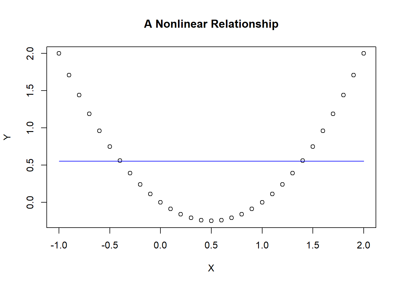
There is an entire section devoted to relaxing the linearity assumption later on, but consider a stark example to illustrate a violation of this assumption. In particular, suppose you consider a simple linear regression model to uncover the relationship between a dependent variable and an independent variable.
\[Y_i=\beta_0+\beta_1X_i+\varepsilon_i\]
However, suppose the true relationship (shown in the figure) is clearly nonlinear, and the blue line in the figure is the estimated (linear) SRF. As the line suggests, it is horizontal suggesting that the linear relationship between Y and X is zero. This doesn’t mean that there is no relationship - because there clearly is. However, our assumption of this relationship being linear is incorrect because the results tell us that there is no linear relationship.

7.5.2 Independence of Errors
Serial correlation exists when an observation of the error term is correlated with past values of itself. This means that the errors are not independent of each other.
\[\varepsilon_t=\rho \varepsilon_{t-1}+\nu_t\]
If this is the case, the model violates the idea that the errors are completely unpredictable. If we would be able to view our past mistakes and improve upon our predictions - why wouldn’t we?12
7.5.3 Equal Variance
The error term must have a constant variance throughout the range of each independent variable because we will soon see that the confidence we place in our estimates are partially determined by this variance. We are unable to change our confidence in the estimates throughout the observed range of independent values - it is one size fits all. Therefore, the size of the errors (i.e., the dispersion in the garbage can) must be constant throughout.

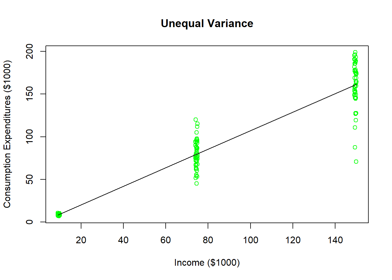
Suppose you wanted to estimate how much of an additional dollar of income the population would spend on consumption.13 Your data set has 50 household observations from each of three annual income levels: $10,000, $75,000, and $150,000 as well as their annual consumption expenditures. As the figure illustrates, households earning around $10,000 a year all have roughly the same consumption level (because they all save very little). As income levels increase, you see more dispersion in consumption expenditures because more income is paired with more options. Households earning $150,000 annually could choose to save a majority of it or even go into debt (i.e., spend more than $150,000). This data could be used to estimate a regression line (illustrated in black), but you can see that the model looks like it does a poorer and poorer job of predicting consumption expenditures as the income levels increase. This means that the forecast errors are increasing as income levels increase, and this is heteroskedasticity. We will briefly come back to potential solutions to this later in the advanced topics section.
7.5.4 Normality of Errors
We know that OLS will produce forecast errors that have a mean of zero as well as a variance that is as low as possible by finding the best fitting straight line. The assumption that these are now the two moments that can be used to describe a normal distribution comes directly from the Central Limit Theorem and the concept of a sampling distribution. Recall that the population error term is zero on average and has some nonzero variance. A random sample of these error terms should have similar characteristics, as well as comprising a normal distribution.