9.1 Nonlinear Models
\[Y_i = \beta_0 + \beta_1 X_{1i} + \beta_2 X_{2i} + \varepsilon_i\]
The regression model we have studied thus far has two main features. First, the model is linear in the coefficients. This important property allows us to estimate the model using OLS. Second the model is linear in the variables. This property imposes a linear relationship between the dependent and independent variables. In other words, the relationship is a straight line.
A linear relationship between the independent and a dependent variable results in a slope that is constant.
\[\beta_1 = \frac{\Delta Y_i}{\Delta X_{1i}}\]
This means that (holding \(X_{2i}\) constant, of course) the expected value of \(Y\) will increase by \(\beta_1\) units in response to any unit-increase in \(X_{1i}\). The same increase occurs on average no matter where in the range of the independent variable you are. Sometimes this assumption is valid if the range of the independent variable is small enough such that a constant slope is appropriate. Sometimes it isn’t. If this assumption is not valid, then we are committing a specification error even if we have included all of the necessary independent variables. The specification error involves the assumption of a linear model.
The types of models we will consider here will be non-linear in the variables but will still be linear in the coefficients. This means that we can still estimate the models using OLS, but we will be extending the model to uncover some highly non-linear relationships between the dependent and independent variables. We will do this by transforming the variables prior to estimation, and the names of these models are given by the types of transformations we perform. We then run a simple OLS estimation on the transformed variables, and back-out the non-linear relationships afterwards. This last bit is what will be new to us, but you will see that it only involves a brief refresher of… calculus.
9.1.1 Derivatives
In calculus, the slope of a function is a simplistic term for it’s derivative. Take for example the very general function \(f(X) = aX^b\). This function uses two parameters (\(a\) and \(b\)) and one variable (\(X\)) to return a number or function value \(f(X)\). If you think about it, this is exactly what the deterministic component of our regression does. When \(b\neq1\), this function is non-linear. Therefore, to determine the slope - the increase in the function value given a unit-increase in \(X\) - we need to take the derivative. The general formula for a derivative is given by
\[\frac{\Delta f(X)}{\Delta X}=abX^{b-1}\]
Note that we have used this derivative formula before, only we used it when \(f(X)=Y\) and the formula was linear (i.e. \(b=1\)) and \(a = \beta\).
\[Y_i = \beta_0 + \beta_1 X_i + \varepsilon_i\]
\[\frac{\Delta Y_i}{\Delta X_i}=\beta_1\]
9.1.2 Why consider non-linear relationships?
The models we will consider below will generally use this extension (and a few other calculus tools) to transform our variables and get at specific non-linear relationships. The reason we do this is to get at the true relationship between the dependent and independent variables. If the relationship is in fact linear, then none of these sophisticated models are necessary. If the relationship is not linear, then linear models are by definition incorrect and will deliver misleading results. The models in this section are therefore used only when the data requires them. Nobody wants to make a model more complicated than it needs to be.
9.1.3 Functional Forms
The sole purpose of introducing a sophisticated functional form into an otherwise straight-forward regression model is because the relationship between a dependent an independent variable is not linear in the data. Recall that a linear relationship is one where the slope is constant. If the slope is constant (say, \(\beta\)), then a one-unit increase in \(X\) will deliver a \(\beta\) unit increase in \(Y\) on average no matter where in the range of X you are. There are a lot of instances in the real world where this doesn’t make sense. Take for example the impact of apartment rental price on its size. One can imagine that if an apartment is small (e.g. 50 sq ft), then one might be willing to pay a lot more for a slight increase in size. If an apartment is ridiculously huge (e.g. 5000 sq ft), then one might not be willing to pay anything for an increase in size. This means that the relationship between apartment rental price and size is conceptually non-linear - the slope is dependent upon the actual size of the apartment. However, if your data has a small range (e.g., between 300 and 400 sq ft), then you might never need to consider a non-linear relationship because a linear one does a good job of approximating the relationship that you observe. This chapter deals with situations where you observe a non-linear relationship in your actual data, so it needs to be modeled.
Once we have established that a relationship is non-linear, we next need to take a stand on what type of non-linear relationship we are attempting to uncover. Answering this question depends upon how you think the slope is going to behave.
Is the slope not constant in unit changes, but constant in percentage changes?
Does the slope qualitatively change? In other words, is there a relationship between a dependent and independent variable that starts out as positive (or negative) and eventually turns negative (or positive)?
Does the slope start out positive or negative and eventually dies out (i.e., goes to zero)?
This chapter details three types of non-linear transformations each designed to go after one of these three scenarios. Non-linear transformations are not one size fits all, so having a good idea of how to handle each type of relationship is essential.
9.1.4 The Log transformation
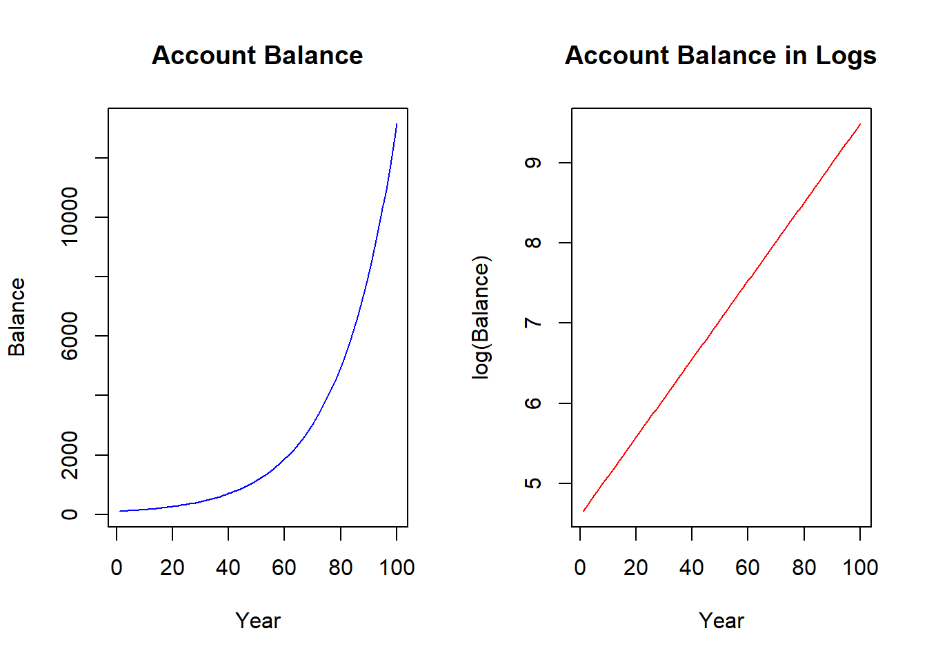
The natural log transformation is used when the relationship between a dependent and independent variable is not constant in units but constant in percentage changes (or growth rates). Imagine putting $100 in a bank at 5 percent interest. If you kept the entire balance in the account, then after one year you will have $105 (a $5 increase), after two years you will have $110.25 (a $5.25 increase), after three years you will have $115.76 (a $5.76 increase), and so on. What is happening is that the account balance is not growing in constant dollar units, but it is growing in constant percentage units. In fact, the balance is said to be growing exponentially. Things like a country’s output, aggregate prices, population all grow exponentially because they build on each other just like the compound interest story.
If we kept our $100 dollars in the bank for a very long time, the balance would evolve according to the figure below on the left. The figure illustrates a non-linear relationship between account balance and time - and the slope is getting steeper as time goes on. While we know that the account balance is increasing by larger and larger dollar increments, we also know that it is growing at a constant five percent. We can uncover this constant percentage change by applying the natural log to the balance - as we did to the right figure. You can see that the natural log function straightens the exponential relationship - so the transformed relationship is linear and ready for our regression model.
The derivative of the log function
The natural log function has a very specific and meaningful derivative:
\[\frac{dln(Y)}{dY} = \frac{\Delta Y}{Y}\]
This formula is actually a generalization of the percentage change formula. Suppose you wanted to know the difference between \(Y_2\) and \(Y_1\) in percentage terms relative to \(Y_1\). The answer is
\[\frac{Y_2 - Y_1}{Y_1} * 100\%\]
Therefore, the only thing missing from the log transformation is the multiplication of \(100\%\), which we can do after estimation.
For example, suppose that you didn’t know the average percentage change (or average growth rate) of your account. If Y was your account balance and X was number of years in the account, then you could estimate what it was. Notice that the slope is 0.05. If you multiply that by \(100\%\) then you have your 5% interest rate back.
R <- lm(log(Y)~X)| (Intercept) | X |
|---|---|
| 4.61 | 0.05 |
Log-log and Semi-log models
Recall that a standard slope is the change in Y over a change in X. Combine this fact with the log of a variable delivers a percentage change in the derivative (provided you multiply by \(100\%\)), and you have several options for which variables you want to consider the logs of. The question you ask yourself is if you want to consider the change of a variable in units or the percentage change of a variable.
Log-log model
A Log-log model is one where both the dependent and the independent variable are logged.
\[ln(Y_i)=\beta_0 + \beta_1 ln(X_i) + \varepsilon_i\]
The slope coefficient \((\beta_1)\) details the percentage change in the dependent variable given a one percent change in the independent variable. To see this, apply the derivative formula above to the entire formula.
\[\frac{dln(Y_i)}{dY} = \beta_1 \frac{dln(X_i)}{dX}\] \[\frac{dln(Y_i)}{dY} * 100\% = \beta_1 \frac{dln(X_i)}{dX} * 100\%\] \[\%\Delta Y_i = \beta_1 \%\Delta X_i\] \[ \beta_1 =\frac{\%\Delta Y_i}{\%\Delta X_i}\]
Semi-log models
Sometimes it makes no sense to take the log of a variable because the percentage change makes no sense. For example, it wouldn’t make sense to take the log of the year in the bank account example above because time is not relative. In other words, a percentage change in time doesn’t make sense. In addition, variables that reach values of zero or lower cannot be logged because the natural log is only defined on positive values. In either case, it would only make sense to not take the log of some of the variables.
A Log-lin model is a semi-log model where only the dependent variable is logged. This is like the case with the bank account example above.
\[ln(Y_i)=\beta_0 + \beta_1 X_i + \varepsilon_i\]
\[\frac{dln(Y_i)}{dY} = \beta_1 \Delta X\] \[\frac{dln(Y_i)}{dY} * 100\% = (\beta_1 * 100\%)\Delta X\] \[\frac{\% \Delta Y}{\Delta X}= \beta_1 * 100\%\] Note that the \(100\%\) we baked into the interpretation is explicitly accounted for in order to turn the derivative of the log function into a percentage change.
A Lin-Log model is a semi-log model where only the independent variable is logged. This might come in handy when you want to determine the average change in the dependent variable in response to a percentage-change in the independent variable.
\[Y_i=\beta_0 + \beta_1 ln(X_i) + \varepsilon_i\]
\[\Delta Y=\beta_1 \frac{dln(X_i)}{X_i}\] \[\Delta Y=\beta_1 \frac{dln(X_i)}{X_i}*\frac{100}{100}\] \[\Delta Y=\frac{\beta_1}{100} \%\Delta X\]
\[\frac{\Delta Y}{\%\Delta X}=\frac{\beta_1}{100} \] Note that the derivation for the lin-log model suggests that you must divide the estimated coefficient by 100 in order to state the expected change in the dependent variable due to a percentage change in the independent variable.
It isn’t ALL OR NOTHING!!!
To be clear, if you have a multiple regression model with several independent variables, you get to treat each independent variable however you wish. In other words, if you log one independent variable, you do not need to automatically log the others. This is especially the case when some can be logged while others cannot. The bottom line is that if you have one of the relationships detailed above with the dependent variable and a single independent variable, then you use the correct derivative form and provide the correct interpretation.
In particular, suppose you had the following model
\[ln(Y_i)=\beta_0 + \beta_1 X_{1i} + \beta_2 ln(X_{2i}) + \varepsilon_i\]
This model is a combination between a log-lin model (with respect to \(X_{1i}\)) and a log-log model (with respect to \(X_{2i}\)). The derivatives are therefore
\[\beta_1 * 100\% = \frac{\% \Delta Y}{\Delta X_1}\]
\[\beta_2= \frac{\% \Delta Y}{\%\Delta X_2}\]
Application
If we ran a regression with hourly wage as the dependent variable and tenure (i.e., years on the job) as the independent variable, then we are estimating the average change in dollars for an additional year of tenure. However, it might be more worthwhile to consider an annual average percentage change in wage as opposed to a dollar change. That is what happens for most people, anyway.
data(wage1,package="wooldridge")

REG <- lm(log(wage) ~ tenure, data = wage1)| Estimate | Std. Error | t value | Pr(>|t|) | |
|---|---|---|---|---|
| (Intercept) | 1.5 | 0.03 | 55.87 | 0 |
| tenure | 0.02 | 0 | 7.88 | 0 |
| Observations | Residual Std. Error | \(R^2\) | Adjusted \(R^2\) |
|---|---|---|---|
| 526 | 0.5 | 0.11 | 0.1 |
The slope estimate gets multiplied by \(100\%\) so we can state that wages increase by \(2\%\) on average for every additional year of tenure.
9.1.5 The Quadratic transformation
A quadratic transformation is used when the relationship between a dependent and independent variable changes direction. The slope can start off positive and become negative (the blue line in the figure), or begin negative and become positive (the red line).
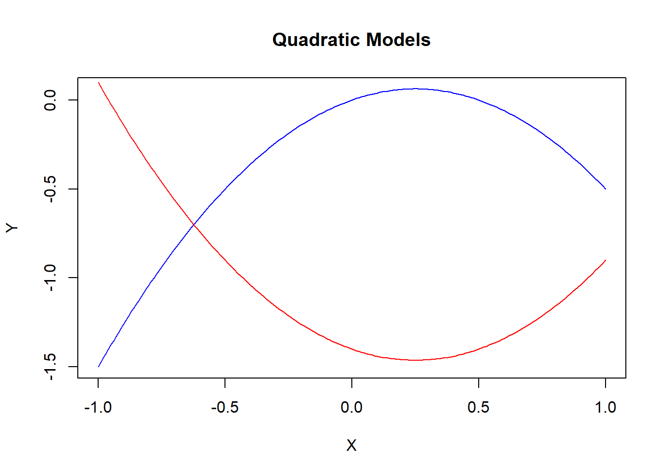
Quadratic models are designed to handle functions featuring slopes that change qualitatively.
\[Y_i = \beta_0 + \beta_1 X_i + \beta_2 X_i^2 + \varepsilon_i\]
Notice that this regression has one variable showing up twice: once linearly and once squared. The regression is still linear in the coefficients, so we can estimate this regression as if the regression contained any two independent variables of interest. In particular, if you defined a new variable \(X_{2i} = X_i^2\), then the model would look like a standard multiple regression.
Once the estimated coefficients are obtained, they are combined to calculate one non-linear slope equation.
\[\frac{\Delta Y}{\Delta X} = \beta_1 + 2\beta_2 X\]
A few things to note about this slope equation.
It is a function of X - meaning that you need to choose a value of the independent variable to calculate a numerical slope. This means you are calculating the expected change in X from a unit increase in X from a particular value.
The slope is increasing or decreasing depending on the values of the coefficients and the independent value of X. The coefficients \(\beta_1\) and \(\beta_2\) are usually of opposite sign. Therefore, the slope is negative if \(\beta_1<0\) and X is small so \(\beta_1 + 2\beta_2 X<0\), or positive if \(\beta_1>0\) and X is small so \(\beta_1 + 2\beta_2 X>0\).
Note: just as in the log transformation, this quadratic transformation does not need to be done to every independent variable in the regression. Only those that are suspected to have a relationship with the dependent variable that changes direction.16
Application
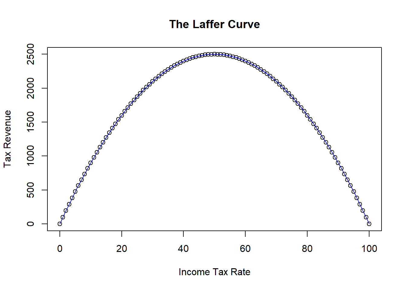
Consider some simulated data illustrating the relationship between tax rates and the amount of tax revenue collected by the government. One can intuitively imagine that the government will collect zero revenue if they tax income at zero percent. However, they will also collect zero revenue if they tax at 100 percent because nobody will work if their entire income is taxed away. Therefore, there should be a relationship between tax rate and tax revenue that looks something like the figure below.
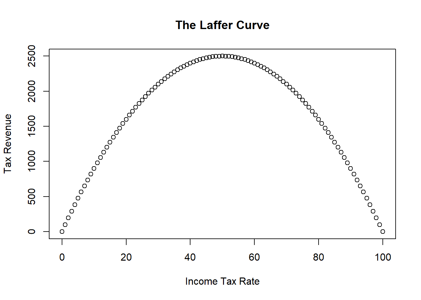
This figure illustrates the infamous Laffer Curve of supply-side economics.17
Suppose you had the data illustrated in the figure. If you assumed a linear relationship between tax revenue and rate, then you will get a very misleading result.
REG <- lm(Revenue ~ Rate)| Estimate | Std. Error | t value | Pr(>|t|) | |
|---|---|---|---|---|
| (Intercept) | 1650 | 151.7 | 10.88 | 0 |
| Rate | 0 | 2.62 | 0 | 1 |
| Observations | Residual Std. Error | \(R^2\) | Adjusted \(R^2\) |
|---|---|---|---|
| 101 | 767.8 | 0 | -0.01 |
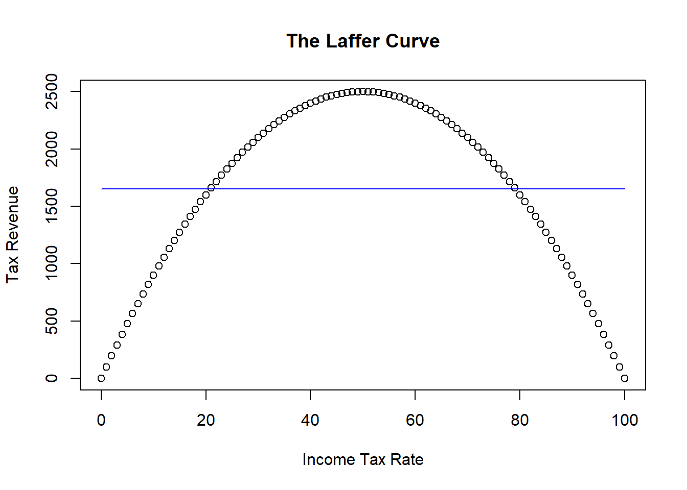
The figure shows that the best fitting straight line is horizontal - meaning that the slope is zero. This linear model would suggest that there is no relationship between tax revenue and tax rate. It is partly true - there is just no linear relationship.
REG <- lm(Revenue ~ Rate + I(Rate^2))| Estimate | Std. Error | t value | Pr(>|t|) | |
|---|---|---|---|---|
| (Intercept) | 0 | 0 | -4.99 | 0 |
| Rate | 100 | 0 | 3.729e+15 | 0 |
| I(Rate^2) | -1 | 0 | -3.853e+15 | 0 |
| Observations | Residual Std. Error | \(R^2\) | Adjusted \(R^2\) |
|---|---|---|---|
| 101 | 0 | 1 | 1 |
9.1.6 The Reciprocal transformation
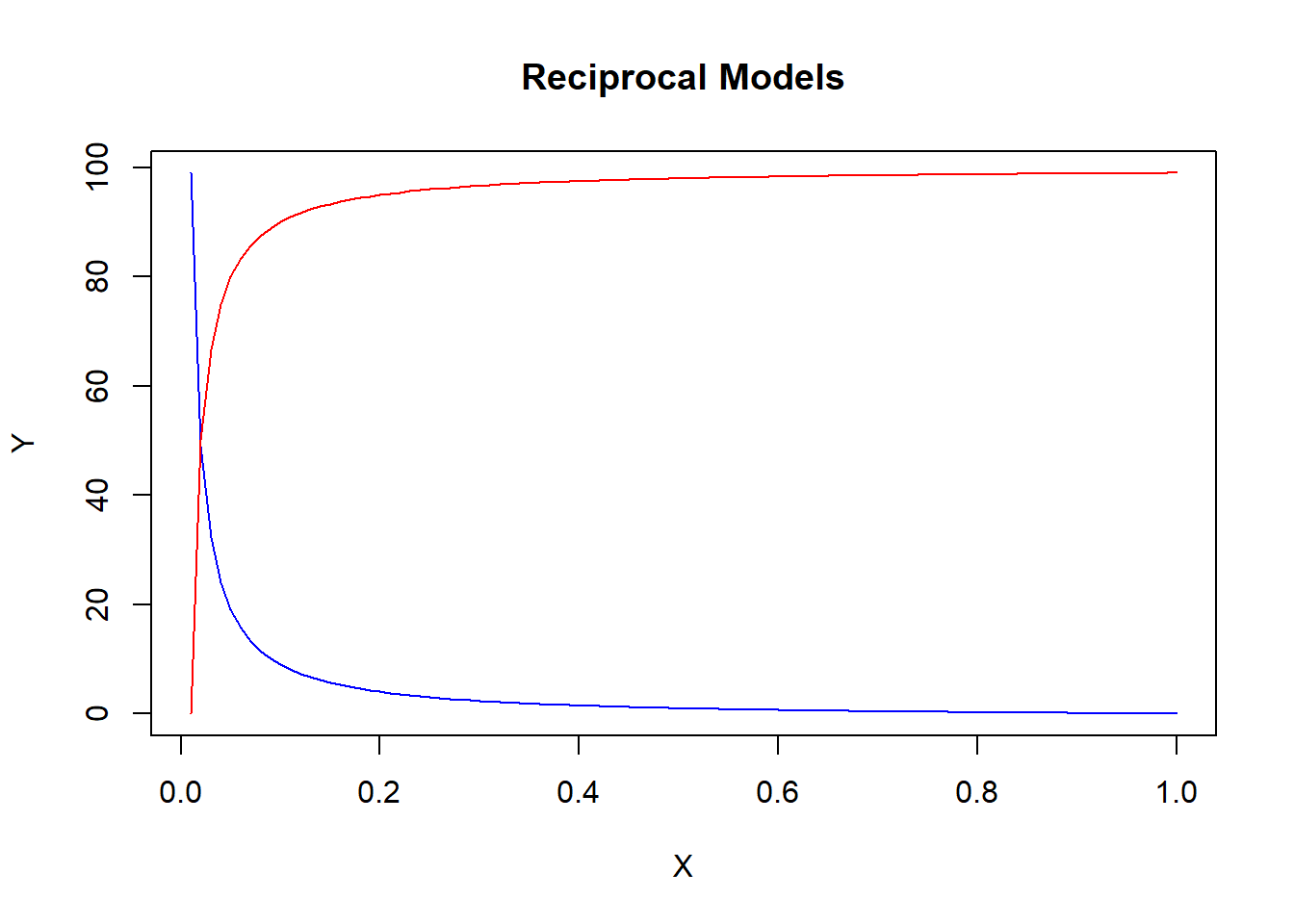
Suppose a relationship doesn’t change directions as much as it dies out.
\[Y_i = \beta_0 + \beta_1 \frac{1}{X_i} + \varepsilon_i\]
As in the quadratic transformation, this model is easily estimated by redefining variables (i.e., \(X_{2i}=1/X_i\)). The slope of this function can be obtained using our standard derivative function and noting that \(1/X_i = X_i^{-1}\)
\[Y_i = \beta_0 + \beta_1 \frac{1}{X_i} + \varepsilon_i\] \[Y_i = \beta_0 + \beta_1 X_i^{-1} + \varepsilon_i\] \[\frac{\Delta Y}{\Delta X} = -\beta_1 X_i^{-2}=\frac{-\beta_1} {X_i^{2}}\]
Notice again that a value of the independent variable is needed to calculate the slope of the function at a specific point. However, as X gets larger, the slope approaches zero. A slope of zero is a horizontal line - and that is when the relationship between Y and X dies out. If \(\beta_1>0\) then the slope begins negative and approaches zero from above (the blue line). If \(\beta_1<0\) then the slope begins positive and approaches zero from below (the red line).
Application
The richer a nation is, the better a nation’s health services are. However, a nation can eventually get to a point that health outcomes cannot improve no matter how rich it gets. This application considers child mortality rates of developing and developed countries and uses the wealth of a country measured by per-capita gross national product (PGNP) to help explain why the child mortality rate is different across countries.
library(readxl)
CM <- read_excel("data/CM.xlsx")

REG <- lm(CM$CM ~ I(1/CM$PGNP))| Estimate | Std. Error | t value | Pr(>|t|) | |
|---|---|---|---|---|
| (Intercept) | 81.79 | 10.83 | 7.55 | 0 |
| I(1/CM$PGNP) | 27273 | 3760 | 7.25 | 0 |
| Observations | Residual Std. Error | \(R^2\) | Adjusted \(R^2\) |
|---|---|---|---|
| 64 | 56.33 | 0.46 | 0.45 |
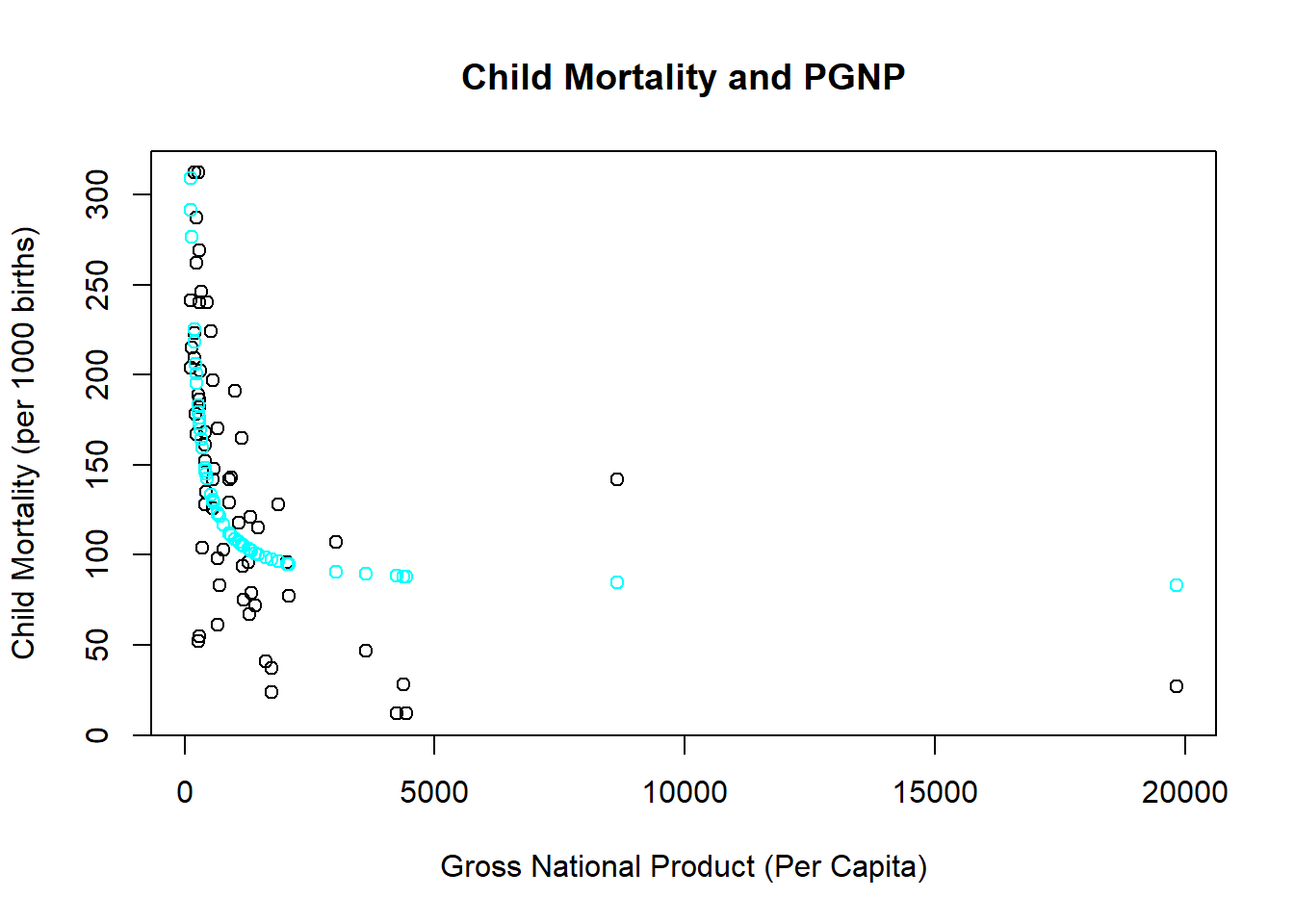
The estimated coefficient is large and positive. However, this isn’t the entire slope, because you need to consider the derivative formula above.
\[\frac{\Delta Y}{\Delta X} = \frac{-27,273} {X_i^{2}}\]
If you wanted to consider the impact on child mortality of making a relatively poor nation richer, you plug a low value for PGNP like 100. If you want to consider a richer nation, consider a larger value like 1000.
\[\frac{\Delta Y}{\Delta X} = \frac{-27,273} {100^{2}} = -2.73\] \[\frac{\Delta Y}{\Delta X} = \frac{-27,273} {1000^{2}} = -0.0273\] These calculations show that increasing the wealth of richer countries has a smaller impact on child mortality rates. This should make sense, and it takes a reciprocal model to capture it.
9.1.7 Conclusion
This section introduced you to three different ways of adding potential non-linear relationships into our model while still preserving linearity in the coefficients. This allows us to retain our OLS estimation procedure, and only requires some calculus steps after estimation to get at our answers.
One take away is that one can easily map out a functional form in theory, but it might not be entirely captured by the data sample. In other words, while we can always tell a story that a relationship might become non-linear eventually, if that extreme range is not in the data then a non-linear relationship isn’t necessary.
On the other hand, if there is a non-linear relationship in the data, then it might be the case that more than one functional form might fit. While it is true that the three transformations handle different right-side behaviors, notice that the left-side of the relationships look quite similar.
Take the figure below for example. We do not have enough data to see if the relationship stays increasing (requiring a log transformation), changes direction (requiring a quadratic transformation), or dies out (requiring a reciprocal transformation). If this is the case then trial and error combined with a lot of care is required.
Which model has the highest \(R^2\)? (Provided that the dependent variable is not transformed.)
Which model makes the most sense theoretically?
What is the differences in the out-of-sample forecasts between models? What is the cost of being wrong?
X <- seq(0,45,1)
Y <- 100 * X - X^2

plot(X,Y,
     main = "Which Relationship is This?",
     xlab = "X",
     ylab = "Y")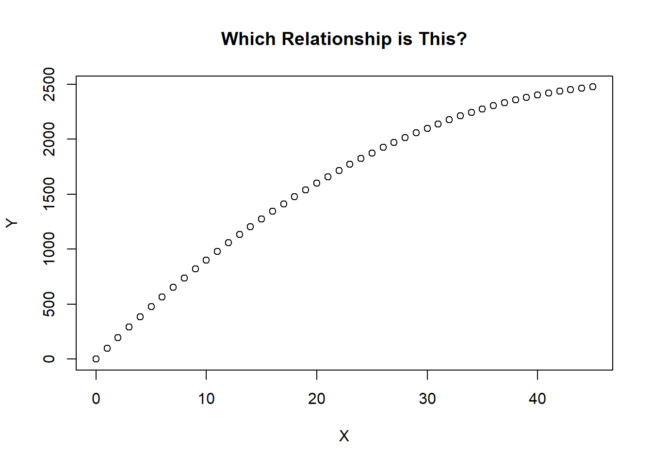
The bottom line is that choosing the wrong non-linear transformation will still lead to some amount of specification bias, but it might not be as much as a linear specification.
For example, you will never be able to look at a quadratic transformation for a dummy variable because when the observations are only 0 and 1, then \(X\) and \(X^2\) are technically the same variable!↩︎
We are using this as an example of a quadratic relationship only - I will spare you my tirade on the detrimental use of this (admittedly intuitive) idea by supply-siders.↩︎