7.3 Ordinary Least Squares (OLS)
Ordinary Least Squares (OLS, for short) is a popular method for estimating the unknown parameters in a linear regression model. OLS chooses the parameters of a linear function by minimizing the sum of the squared differences between the observed dependent variable (values of the variable being observed) in the given data set and those predicted by the linear function.
To illustrate this, consider a sample of observations and a PRF:
\[Y_i=\beta_0+\beta_1X_i+\varepsilon_i\]

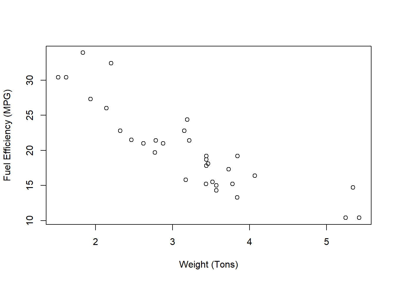
Look at the figure and try to imagine the best fitting straight line that goes through all observations in the scatter plot. This line has two features: and intercept term \((\hat{\beta}_0)\) and a slope term \((\hat{\beta}_1)\). Which values would you assign?
We can go about this a little more formally. First, if we had values for \(\hat{\beta}_0\) and \(\hat{\beta}_1\), then we can determine the residual (error) for each pair of \(Y_i\) and \(X_i\).
\[e_i = Y_i - (\hat{\beta}_0 + \hat{\beta}_1X_i)\]
We can sum across all observations to get the total error
\[\sum_{i}e_i = \sum_{i}(Y_i - \hat{\beta}_0 - \hat{\beta}_1X_i)\]
The problem we face now is that error terms can be both positive and negative. That means they will start to wash each other out when we sum them up and we therefore get an incomplete measure of the total error. To prevent the positive and negative error terms from washing each other out, we square each of the terms. This makes the negative errors positive, while the positive errors stay positive.9
\[\sum_{i}e^2_i = \sum_{i}(Y_i - \hat{\beta}_0 - \hat{\beta}_1X_i)^2\]
Notice that this function now states that we can calculate the sum of squared errors for any given values of \(\hat{\beta}_0\) and \(\hat{\beta}_1\). We can therefore find the best values of \(\hat{\beta}_0\) and \(\hat{\beta}_1\) that deliver the lowest sum of squared errors. The line that delivers the lowest squared errors is what we mean by the best line.
\[min\sum_{i}e^2_i = min_{(\hat{\beta}_0,\hat{\beta}_1)}\sum_{i}(Y_i - \hat{\beta}_0 - \hat{\beta}_1X_i)^2\]
This function is called an objective function, and we can minimize the sum of squared errors by taking first-order conditions (i.e., the derivative of the objective function with respect to \(\hat{\beta}_0\) and \(\hat{\beta}_0\)).
\[\hat{\beta}_1=\frac{\sum_i (X_i-\bar{X})(Y_i-\bar{Y})}{\sum_i(X_i-\bar{X})^2}=\frac{cov(X,Y)}{var(X)}\]
\[\hat{\beta}_0=\bar{Y}-\hat{\beta}_1\bar{X}\]
Where a ‘bar’ term over a variable represents the mean of that variable (i.e., \(\bar{X}=\frac{1}{n}\sum_iX_i\))
These two equations are important. The first equation states that the slope of the line equation \((\hat{\beta}_1)\) is equal to the ratio between the covariance of Y and X and the variance of X. Remember that a covariance measures how two variables systematically move together. If they tend to go up at the same time, then they have a positive covariance. If they tend to go down - a negative covariance. If they do not tend to move together in any systematic way, then they have zero covariance. This systematic movement is precisely what helps determine the slope term. The second equation states that with \(\hat{\beta}_1\) determined, we can determine \(\hat{\beta}_0\) such that the regression line goes through the means of the dependent and independent variables.
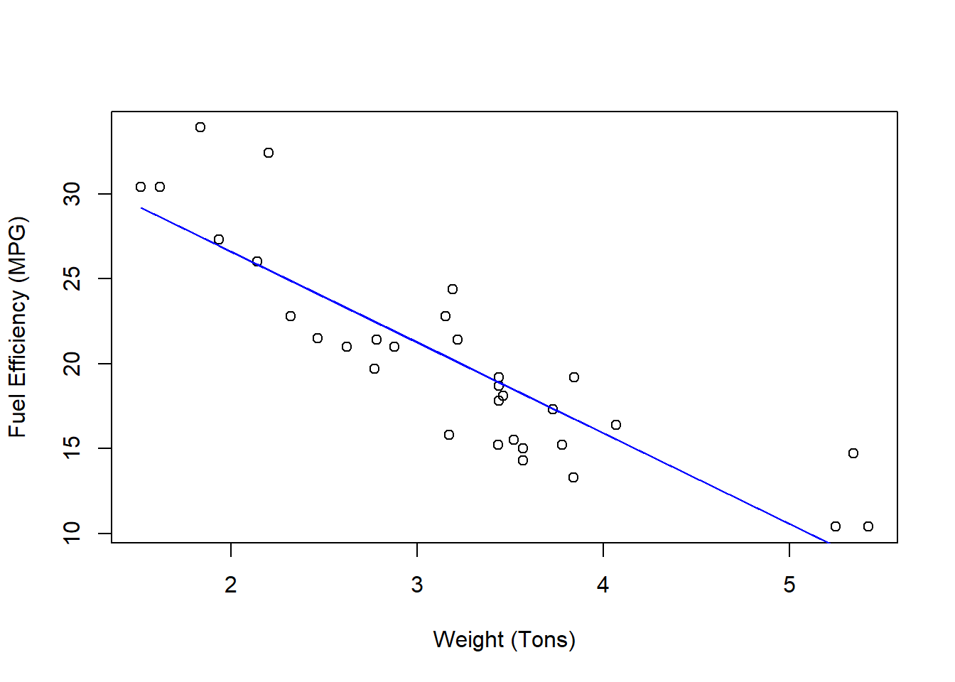
Lets see what these estimates and the resulting regression line look like.
REG <- lm(mpg~wt,data = mtcars)
coef(REG)
## (Intercept) wt
## 37.285126 -5.344472plot(mtcars$wt,mtcars$mpg,
xlab = "Weight (Tons)",
ylab = "Fuel Efficiency (MPG)")
lines(mtcars$wt,fitted(REG),col='blue')
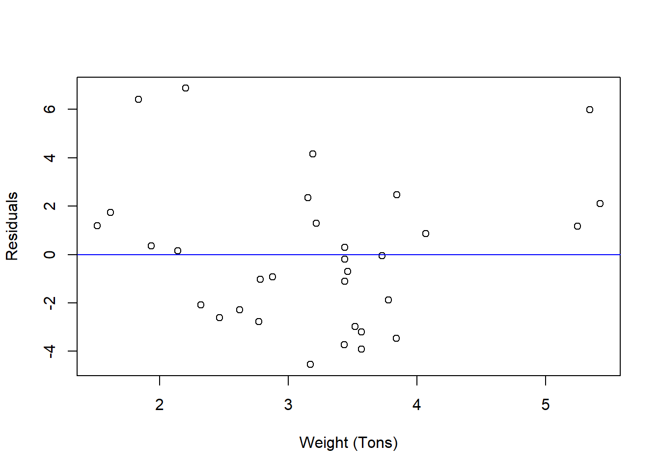
Now you probably imagined a line that looked kinda like this, but we know that this line (with these coefficients) is the absolute best line that minimizes the total difference between the observations (the dots) and the predictions (the line). Any other line we could draw would have a larger sum of squared errors. We can see what this difference looks like by looking at the residuals.
plot(mtcars$wt,residuals(REG),
     xlab = "Weight (Tons)",
     ylab = "Residuals")
abline(h = 0,col="blue")
Notice that these residual values are distributed both above and below the zero line. If you were to sum them all up - then you get zero ALWAYS. It is what the mathematical problem is designed to do!
\[\sum_ie_i=0\]
This mathematical outcome is actually important. First, if the residuals or forecast errors sum up to zero, then that means that they have a mean that is also 0 \((\bar{e}=0)\). This means that they are zero on average, so the expected value is zero!
\[E[e_i]=0\]
If the expected value of the forecast error is zero, then this means that our regression line is correct on average. If we think about it, this is the best we can ask for out of a regression function.
7.3.1 B.L.U.E.
OLS is a powerful estimation method that delivers estimates with the following properties.
They are the BEST in a minimized mean-squared error sense. We just showed this.
They are LINEAR insofar as the OLS method can be quickly used when the regression model is a linear equation.
They are UNBIASED meaning that the sample estimates are true estimates of the population parameters.
Therefore, BEST, LINEAR, UNBIASED, ESTIMATES is why the output of an OLS method is said to be B.L.U.E.
Note: this is where the sum of squared errors comes in.↩︎