9.3 Heteroskedasticity

Another violation of our regression assumptions is that of heteroskedasticity. Pure homoskedasticity occurs when the variance of the error term is constant:

\[VAR (\varepsilon_i ) = \sigma^2 \;(i = 1, 2, ...,N)\]

With heteroskedasticity, this error term variance is not constant. In other words, the distribution of the error term now depends on which values are being considered.

\[VAR (\varepsilon_i ) = \sigma_i^2 \;(i = 1, 2, ...,N)\]

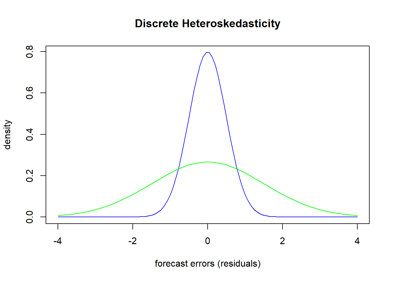
An example of heteroskedasticity would be one where you could break the forecast errors into two discrete groups. Suppose you have the results of a statistics test and you considered the forecast errors for males and females separately.

One gender has forecasts errors that comprise the green distribution while the other gender has forecast errors that comprise the blue distribution. Both distributions have zero mean, but the differences in distributions suggest that there is more volatile forecast errors for the green distribution than the blue. This is a problem because the standard deviation of the entire garbage can is used to deliver statistical inference on the precision of the model. If we were to say that females and males comprised the blue and green distributions respectively, then this is saying that the model does a much better job at predicting female test scores than male test scores. Since our precision is an average of these two results, it actually indicates that we do worse on females and better on males than what is truly going on.

9.3.1 Pure versus Impure Heteroskedasticity

We can categorize heteroskedasticity depending on whether it is due to a model misspecification (on the part of the researcher) or if it is simply a force of nature. Heteroskedasticity is said to be impure if it is due to a model misspecification. If this is the case, then a change in the model might very well remove the heteroskedasticity and that’s that. If heteroskedasticity is said to be pure, then it is the result of the true relationship in the data and no change in model specifications will correct it. If this is the case, then more sophisticated methods are called for.

9.3.2 Consequences of Heteroskedasticity

Heteroskedasticity has two consequences:

OLS is no longer the minimum variance estimator (of all the linear unbiased estimators). In other words, OLS is no longer BLUE.
OLS estimates of the standard errors are biased. The bias is typically negative, meaning that OLS underestimates the standard errors, overestimates the t-scores, and makes hypothesis tests more likely to be rejected.

Note that while heteroskedasticity underestimates the standard errors, it does not deliver bias on the estimates themselves. So it’s not a problem of the estimates, its that the estimates appear more significant due to heteroskedasticity.

9.3.3 Detection

Before using any test for heteroskedasticity, ask the following:

Are there any obvious specification errors? If so, then we might be able to correct impure heteroskedasticity without even knowing it. Fix those before testing!
Is the subject of the research likely to be afflicted with heteroskedasticity? Not only are cross-sectional studies the most frequent source of heteroskedasticity, but cross-sectional studies with large variations in the size of the dependent variable are particularly susceptible
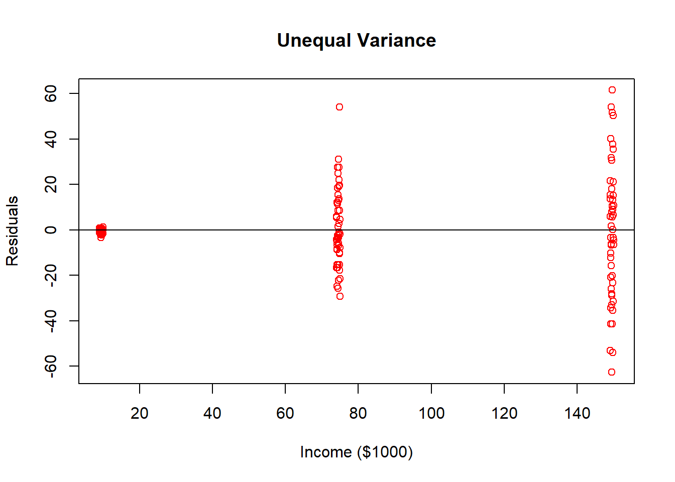
Does a graph of the residuals show any evidence of heteroskedasticity? Specifically, plot the residuals against the independent variables. If it appears that the dispersion of the error term is in any way proportional to the independent variables, then it could indicate a problem as well as a solution.

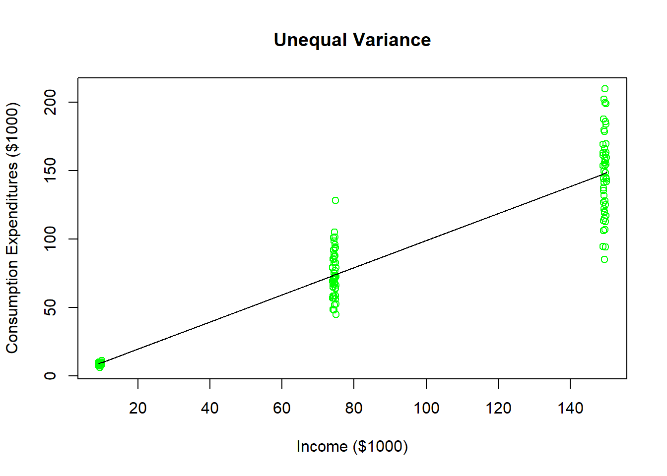
A clear example of how the forecast error variance can be proportional to an independent variable is to return to a previous scenario where we tried to estimate an individuals consumption based on their income levels.

Your data set has 50 household observations from each of three annual income levels: $10,000, $75,000, and $150,000 as well as their annual consumption expenditures. As the figure illustrates, households earning around $10,000 a year in income all have roughly the same consumption level (because they all save very little). As income levels increase, you see more dispersion in consumption expenditures because more income is paired with more options. Households earning $150,000 annually could choose to save a majority of it or even go into debt (i.e. spend more than $150,000). This data could be used to estimate a regression line (illustrated in black), but you can see that the model looks like it does a poorer and poorer job of predicting consumption expenditures as the income levels increase.

If we were to examine the forecast errors of this regression and plot them with income, you will see that the dispersion in indeed proportional to income.

A formal test for heteroskedasticity that we will focus on is the Park test. The Park test is simple but less general than another test called the White test, but the concepts are similar.

A Park test is a formal way of testing if the variance of the residual term is in fact proportional to an independent variable.

Run the initial regression and obtain the residuals $(e_i)$.
Use the log of the squared residuals as the dependent variable for an auxiliary regression with the the independent variable on the right hand side.

\[ ln( e_i^2) = a_0 + a_1 X_i + u_i\]

Test the null hypothesis that $a_1 = 0$. If you reject the null, then you have formal evidence that the variance of the residual term is related to the independent variable.

# A Park test:

EPS <- log(residuals(REG)^2)

PARK <- lm(EPS ~ X)

library(lmtest)
coeftest(PARK)

## 
## t test of coefficients:
## 
##               Estimate Std. Error t value  Pr(>|t|)    
## (Intercept) -0.9867853  0.3508284 -2.8127  0.005579 ** 
## X            0.0492734  0.0036317 13.5676 < 2.2e-16 ***
## ---
## Signif. codes:  0 '***' 0.001 '**' 0.01 '*' 0.05 '.' 0.1 ' ' 1

The results from the Park test suggest that the variance in the forecast errors of consumption are in fact related to income.

9.3.4 Remedies

There are two remedies for heteroskedasticity, and they primarily depend upon whether or not the heteroskedasticity is pure or not.

First, if we are dealing with impure heteroskedasticity then a model re-specification might resolve the issue. If we consider the consumption - income application above, it is fairly well known that including another value such as wealth might help explain dimensions of consumption that income cannot. It might also be better to cast the model in a log-log form so we are looking at percentage changes in income as opposed to absolute changes. Either one of these proposed changes to the model could bring the model closer to a correct specification which could have the added benefit of removing heteroskedasticity.

Second, if we are dealing with pure heteroskedasticity then the issue will not go away no matter how we specify the model. In this case, there are Heteroskedasticity-corrected standard errors. The specifics of this procedure goes a tad beyond the scope of our class, but it corrects the standard errors of a regression in order to compensate for the negative bias caused by heteroskedasticity. These standard errors can be used for all inference of the model.

The code below is what is known as a heteroskedasticity correction. It displays the original coefficient estimates from our model, but alters the standard errors to correct for heteroskedasticity.

coeftest(REG,vcov = hccm)

## 
## t test of coefficients:
## 
##             Estimate Std. Error t value Pr(>|t|)    
## (Intercept) 0.020031   1.317722  0.0152   0.9879    
## X           0.990395   0.030770 32.1871   <2e-16 ***
## ---
## Signif. codes:  0 '***' 0.001 '**' 0.01 '*' 0.05 '.' 0.1 ' ' 1