4.4 The Punchline
Once you determine a sample size \((n)\), you get one random draw from the appropriate sampling distribution.
The distribution is approximately normal
The mean is \(\mu\)
The standard deviation \(\sigma/\sqrt{n}\)
What does this buy us? The answer is everything if we want to apply any form of confidence (i.e., stating a probability of occurring).
The reason is that the normal distribution has a lot of useful properties.
The distribution is symmetric. The shape of the distribution to the right of the mean is identical to the shape of the distribution to the left of the mean.
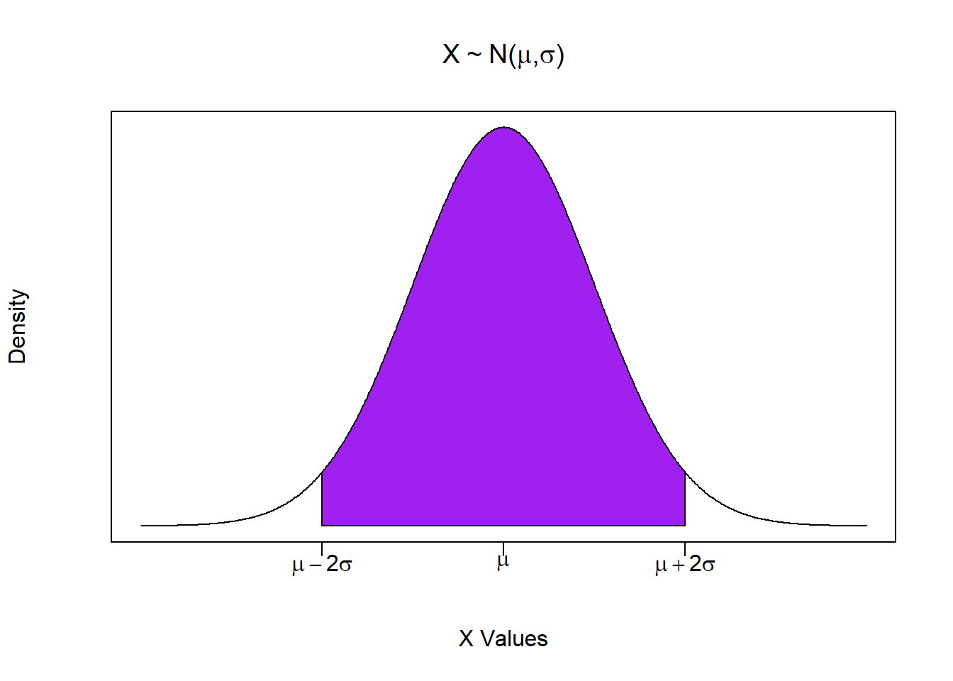
Approximately 95% of all possible outcomes are within 2 standard deviations of the mean.
To illustrate these two properties, consider the generic normal distribution illustrated below. You can easily see the symmetry of the distribution, while the shaded area represents 95% of the distribution. In probability terms, 95% of the area of the probability distribution means that there is a 95% chance of drawing a value within this range.

So what does this really buy us? Consider the application above about the Philadelphia policy where we would have in reality have no idea what the population parameters \((\mu,\;\sigma)\) are, or what the population distribution even looks like. However, the CLT says that if we decide on a sample size \(n\), then we will draw from a sampling distribution that is a normal distribution with mean \(\mu\) and standard deviation \(\sigma / \sqrt{n}\).

So what we know is that once we draw a random sample and construct a sample mean, we can say with 95% confidence that that sample mean was drawn from the shaded region of the above distribution. We know what the sample mean value is because we just calculated it. What we don’t know is what \(\mu\) is. However, we can construct a probabilistic range (a confidence interval) around where we think this population parameter lies. This is where we are going next.