5.3 What to do when we do not know \(\sigma\)
In most instances, if we know nothing about the population parameter \(\mu\) then we know nothing about any of the other parameters (like \(\sigma\)). In this case, we are forced to use our best guess of \(\sigma\). Since we are assuming that our sample has the same characteristics of the population, then our best guess for \(\sigma\) is the sample standard deviation \(S\).
Put plainly, we substitute the statistic (\(S\)) for the population parameter (\(\sigma\)). Because \(S\) is an estimate of \(\sigma\), this will slightly change our probability distribution. In particular, If \(\bar{X}\) is normally distributed as per the CLT, then a standardization using \(S\) instead of \(\sigma\) is said to have a t distribution with \(n-1\) degrees of freedom
\[t=\frac{\bar{X}-\mu}{(S/\sqrt{n})}\]
Note that this looks almost exactly like our Z transformation, only with \(S\) replaced for \(\sigma\). However, this statistic is said to be drawn from a distribution with \(n-1\) degrees of freedom. We mentioned degrees of freedom before, and we stated that we lose a degree of freedom when we build statistics on top of each other. In other words, we lose a degree of freedom for every statistic we use to calculate another statistic. Consider the standard deviation equation needed to calculate \(S\).
\[S = \sqrt{\frac{1}{n-1} \sum_{i=1}^n(X_i-\bar{X})^2}\]
The equation states that the sample mean \((\bar{X})\) is used to calculate the sample standard deviation. This means one statistic is used to calculate a subsequent statistic… and that is why we lose one degree of freedom.
5.3.1 t distribution versus Z distribution…
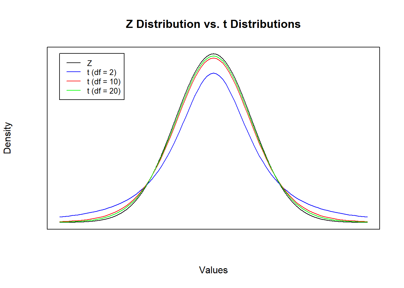
A t distribution and Z distribution have very much in common: they are both symmetric, both centered at a mean of 0, and both sum to one (because they are both probability distributions). The main difference is that a t-distribution has fatter tails than a Z distribution, and the fatness of the tails depends on the degrees of freedom (which in turn depends on the sample size).
The figure below compares the standard normal (Z) distribution with several t distributions that differ in degrees of freedom. Notice that tail thickness of the t distributions are inversely related to sample size. As the the degrees of freedom get larger (i.e., the larger the sample size), the closer the t distribution gets to the Z distribution. This is because as n gets larger, \(S\) becomes a better estimate of \(\sigma\).

\[\bar{X}-Z_{\frac{\alpha}{2}}\frac{\sigma}{\sqrt{n}} \leq \mu \leq \bar{X}+Z_{\frac{\alpha}{2}}\frac{\sigma}{\sqrt{n}}\]
\[\bar{X}-t_{(\frac{\alpha}{2},df=n-1)}\frac{S}{\sqrt{n}} \leq \mu \leq \bar{X}+t_{(\frac{\alpha}{2},df=n-1)}\frac{S}{\sqrt{n}}\]
In a nutshell, the only difference encountered when not knowing \(\sigma\) is that we have a slightly different probability distribution (which requires knowing the degrees of freedom and uses a different R command). The new R commands are qt and pt which requires degrees of freedom but otherwise has all of the same properties of qnorm and pnorm discussed above.
pt(q, df, lower.tail = TRUE)
qt(p, df, lower.tail = TRUE)
5.3.2 Application 4
Suppose you manage a call center and just received a call from Quality Control asking for the average call length at your facility. They are asking for the average call length in the population, so the best you can do is provide a confidence interval around this population parameter. You select a random sample of 50 calls from your facility and calculate a sample average of 5.8 minutes and a sample standard deviation of 2.815 minutes.
\[\bar{X}=5.8, \quad n=50, \quad S=2.815\]
Calculate a 95% confidence interval around the population average call length.
Xbar = 5.8
n = 50
df = n-1
S = 2.815
alpha = 0.05
t = qt(alpha/2,df,lower.tail = FALSE)
(left = Xbar - t * S / sqrt(n))
## [1] 4.999986(right = Xbar + t * S / sqrt(n))## [1] 6.600014With 95% confidence, the population average call length is between 5 minutes and 6.6 minutes.
As before, if we want to change our level of confidence then we change \(\alpha\) and recalculate the t statistic. Notice that the relationship remains that a lower confidence level delivers a narrower confidence interval.
alpha = 0.01 # increase confidence to 99%
t = qt(alpha/2,df,lower.tail = FALSE)
(left = Xbar - t * S / sqrt(n))
## [1] 4.733108(right = Xbar + t * S / sqrt(n))## [1] 6.866892alpha = 0.10 # decrease confidence to 90%
t = qt(alpha/2,df,lower.tail = FALSE)
(left = Xbar - t * S / sqrt(n))## [1] 5.132563(right = Xbar + t * S / sqrt(n))## [1] 6.467437